8.1 Wigner Equation

The transient Wigner equation with relaxation time scattering is

$$\frac{\partial}{\partial t} f(x,k,t) + \frac{\hbar k}{m^*} \frac{... ...,t) + \int V_{\mathrm{w}}(x, k - k') f(x, k', t) dk' + \mathrm{Rel}[f] = 0 .$$ (8.1)

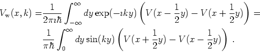
Here $f(x, k, t)$ is the 1-D Wigner function at position $x$, wavenumber $k$ and position $t$. The non-local Wigner potential $V_{\mathrm{w}}(x,k)$ is calculated from the real potential energy $V(x)$ by

$$\begin{gather*}\begin{split}V_{\mathrm{w}}(x,k) =& \frac{1}{2\pi\imath\hbar} \in... ...(V(x + \frac{1}{2}y) - V(x - \frac{1}{2} y)\right) . \end{split}\end{gather*}$$ (8.2)

In Equation 8.1 $\mathrm{Rel}[f]$ denotes the term for relaxation time scattering, that is

$$\mathrm{Rel}[f] = \frac{1}{\tau} \left( f(x,k,t) - f_{\mathrm{eq}}(x,k,t) \frac{n(x,t)}{n_{\mathrm{eq}}(x,t)} \right) .$$ (8.3)

Here $\tau$ denotes the relaxation time, $n$ denotes carrier density

$$n(x) = \frac{1}{2 \pi} \int f(x,k) dk .$$ (8.4)

and $f_{\mathrm{eq}}$ denotes the equilibrium solution. Assuming that the doping is the same in the left and the right electrode we define $f_{\mathrm{eq}}$ as the solution of Equation 8.1 under zero bias (and relaxation time scattering excluded).

Note the factor $1/2 \pi$ which comes from the Wigner transformation of the density matrix trace operation.

The Wigner equation has to be supplemented with suitable boundary conditions. It is of first order in $x$, hence a possibility is to specify the solution on one side of the simulation domain. We used inflow boundary conditions: these are of Dirichlet type in Wigner phase space and specify the incoming flow on the left and on the right contacts. Hence half of the boundary conditions is given on the left, half is given on the right boundary. We assume that even under bias, the distribution in the leads is in equilibrium and the incoming part of the distribution at the contacts is given by this equilibrium distribution. The equilibrium distribution is given by a Fermi-Dirac distribution which poses the boundary conditions:

$$f_L(k > 0) = f_R(k < 0) = \mathcal{FD}(T_L,k) .$$ (8.5)

The Fermi level is correct when the carrier concentration equals the doping density.

We allow the effective mass $m^{*}$ to be a space dependent parameter. This is only an approximation to the Wigner transformation of the term $\partial_x \frac{1}{m^*(x)} \partial_x$ in the Schrödinger equation and is known as ``Frensley's model'' or as ``classical approximation''. The correct term as obtained by Wigner transformation leads to a convolution integral and is treated in [TOM91], [MH94].