Next: 1.4 Organic Light-Emitting Diodes
Up: 1. Introduction
Previous: 1.2 Organic Semiconductor Physics
Subsections
The incoherent dynamics of carriers as well as excitons can be described by a
master equation,
 |
(1.2) |
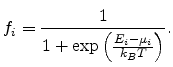
with  denoting the occupation probability of state
  and
and
 the electron or hole transition rate of the hopping process between the occupied
state to empty state
the electron or hole transition rate of the hopping process between the occupied
state to empty state  . Defining
  as the
chemical potential at the position of state and
as the
chemical potential at the position of state and  as the energy of state
, the occupation probability is
given by the Fermi-Dirac distribution function
as the energy of state
, the occupation probability is
given by the Fermi-Dirac distribution function
 |
(1.3) |
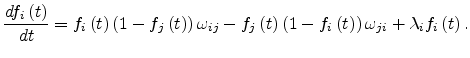
Assuming no correlations between the occupation probability of different
localized states, the steady-state current between these two sites is
given by
![$\displaystyle I_{ij}=q\left[f_i\left(t\right)\left(1-f_j\left(t\right)\right)\omega_{ij}-f_j\left(t\right)\left(1-f_i\left(t\right)\right)\omega_{ji}\right].$](img104.png) |
(1.4) |
Substituting the Miller-Abrahams rate (1.1) in (1.4) the current becomes
![$\displaystyle I_{ij}=\frac{q\nu_0\exp\left(-2\alpha R_{ij}-\frac{\mid E_i-E_j\m...
...\left[\frac{E_i-\mu_i}{2k_BT}\right]\cosh\left[\frac{E_j-\mu_j}{2k_BT}\right]}.$](img105.png) |
(1.5) |
In the case of low electric field, resulting in a small voltage drop over a
single hopping distance (
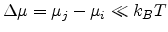 ), the following
conductance is obtained
), the following
conductance is obtained
![$\displaystyle \sigma_{ij}=\frac{I_{ij}}{\Delta\mu}\propto\exp\left[-2\alpha\mid...
...j}\mid-\frac{\mid E_i-\mu\mid+\mid E_j-\mu\mid+\mid E_i-E_j\mid}{2k_BT}\right].$](img107.png) |
(1.6) |
Here
 . This expression was introduced in 1960 by
Miller and Abrahams [7] and is often referred as the Miller-Abrahams
conductance. Equation (1.6) has an important implication. Even if the energies are
moderately distributed, the exponential dependence of
. This expression was introduced in 1960 by
Miller and Abrahams [7] and is often referred as the Miller-Abrahams
conductance. Equation (1.6) has an important implication. Even if the energies are
moderately distributed, the exponential dependence of
 on these
energies makes them enormously broadly distributed. This can be used to reduce
the computations of the effective properties of the network, since the
broadness of the distribution of
implies that there are many
small conductances that can be removed from the network. This resulting network
is called the reduced network [13].
on these
energies makes them enormously broadly distributed. This can be used to reduce
the computations of the effective properties of the network, since the
broadness of the distribution of
implies that there are many
small conductances that can be removed from the network. This resulting network
is called the reduced network [13].
Miller and Abrahams [7] were the first to calculate the hopping conductivity  of
semiconductors using reduced networks. They assumed that the statistical
distribution of the resistances depends only on
of
semiconductors using reduced networks. They assumed that the statistical
distribution of the resistances depends only on  and not on the site
energies. This was justified because the experimental data for some
semiconductors indicated that the impurity conduction exhibits a well-defined
activation energy. But Mott [16] pointed out that the exponential dependence of the
resistances on the site energies can not be ignored in most cases. When a carrier
close to the Fermi energy hops away over a distance
and not on the site
energies. This was justified because the experimental data for some
semiconductors indicated that the impurity conduction exhibits a well-defined
activation energy. But Mott [16] pointed out that the exponential dependence of the
resistances on the site energies can not be ignored in most cases. When a carrier
close to the Fermi energy hops away over a distance  with an energy
  , it has
 sites to choose from, where
  is the site density function. In general,
the carrier will jump to a site for which is as small as
possible. The constraint to find a site within a range
is the site density function. In general,
the carrier will jump to a site for which is as small as
possible. The constraint to find a site within a range
 is given by
 . Substituting
this relation into (1.6) yields
. Substituting
this relation into (1.6) yields
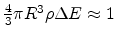
![$\displaystyle G\propto \exp\left[-2\alpha R-\frac{1}{k_BT\left(4/3\right)\pi R^3\rho}\right].$](img114.png) |
(1.7) |
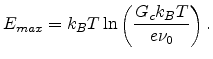
The optimum conductance is obtained by maximizing with respect to the hopping
distance as
![$\displaystyle G\propto\exp\left[-\left(\frac{T_1}{T}\right)^{1/4}\right],$](img115.png) |
(1.8) |
with
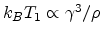 .
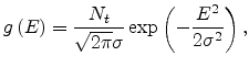
Much theoretical work has been done by investigating the mobilities of organic
semiconductors within the framework of GDM [9]. Non-crystalline
organic solids, such as molecularly doped crystals, molecular glasses, and
conjugated polymers, are characterized by small mean free paths for the
carriers, as a result of the high degree of disorder present in the organic
system. Therefore, the elementary transport step is the charge transfer between
adjacent elements, which can either be molecules participating in
transport or segments of a polymer separated by topological defects. These
charge transporting elements are identified as sites whose energy are subjected
to a Gaussian distribution
.
Much theoretical work has been done by investigating the mobilities of organic
semiconductors within the framework of GDM [9]. Non-crystalline
organic solids, such as molecularly doped crystals, molecular glasses, and
conjugated polymers, are characterized by small mean free paths for the
carriers, as a result of the high degree of disorder present in the organic
system. Therefore, the elementary transport step is the charge transfer between
adjacent elements, which can either be molecules participating in
transport or segments of a polymer separated by topological defects. These
charge transporting elements are identified as sites whose energy are subjected
to a Gaussian distribution
where  is the energy measured relative to the center of the density of
states and
is the energy measured relative to the center of the density of
states and  is the standard deviation of the Gaussian distribution. Within this distribution, all the states are localized. The
choice of such distribution was based on the Gaussian profile of the excitonic
absorption band, as well as on the recognition that the polarization energy is
determined by a large number of internal coordinates, which vary randomly by a
small amount, so the central limit theorem of statistics holds.
is the standard deviation of the Gaussian distribution. Within this distribution, all the states are localized. The
choice of such distribution was based on the Gaussian profile of the excitonic
absorption band, as well as on the recognition that the polarization energy is
determined by a large number of internal coordinates, which vary randomly by a
small amount, so the central limit theorem of statistics holds.
The Gaussian disorder model has been treated by the Monte Carlo simulation
technique based on the Miller Abraham equation [9]. In this simulation
charge transport is described as an incoherent random walk. The carriers start
their motion from randomly chosen sites at one of the boundaries of the system
sample. Their trajectories are specified from the constraint that the
probability for a carrier to jump between two transport sites is
With this technique, TOF measurements can be simulated [9], in which
mobility is derived from the mean arrival time of the carrier at the end of the
sample and from their mean displacement. The predictions made concern the
temperature and electric field dependence of the mobility.
In the Gaussian disorder model, the strength of electronic coupling among sites
is split into separate contributions from the relevant sites, each obtained
from a Gaussian probability density. However, the choice for the off-diagonal
disorder of a Gaussian distribution is not theoretically sustained unlike in
the case of energy disorder, and a more realistic way of representing geometric
disorder has been pursued. One of such attempt is described in [14], in
which an alternative approach comprising positional and orientation disorder is
introduced via fluctuations in the bonds adjoining the various transport sites
rather than site fluctuations. This model gets rid of the unnecessary
corrections between hops and results in overestimating the contribution of the
log hops.
In particular, Gartstein and Conwell's [14] Monte Carlo simulations of hopping
with the elementary jump rate described by 1.1, but in which
where
 is a uniformly distributed random variable. In this way,
the different bonds of a given site with its
neighbors are uncorrelated.
is a uniformly distributed random variable. In this way,
the different bonds of a given site with its
neighbors are uncorrelated.
Another approach for the description of positional disorder was presented by
Hartenstein [15], and was also based on Monte Carlo simulations of transport
in a dilute lattice. This treatment employs the GDM, but without the need for
defining a distribution function for the electronic coupling between different
sites. In this case the hopping sites having the nearest neighbors were
grouped in clusters whose size depends on the random intercluster distances,
but ignores any contribution from the random orientation of the transporting
elements. Nevertheless, the model is adequate for low dopant concentrations for
which there are large fluctuations in the intersite distances.
Ambegaokar and coworkers argued that an accurate estimate of is the critical
percolation conductance  [17], which is the largest value of the conductance
such that the subnet of the network with
[17], which is the largest value of the conductance
such that the subnet of the network with
 still contains a
conducting sample-spanning cluster. They divided the network into three
parts.
First, a set of isolated clusters of high conductivity where each cluster
consists of a group of sites connected together by conductances
still contains a
conducting sample-spanning cluster. They divided the network into three
parts.
First, a set of isolated clusters of high conductivity where each cluster
consists of a group of sites connected together by conductances
 ;
Second, a small number of resistors with
;
Second, a small number of resistors with  of order , which
connect together a subset of high conductance clusters to form the
sample-spanning cluster, called the critical subnetwork, essentially
the same as the static limit of the reduced network discussed above;
and third, the remaining resistors with
of order , which
connect together a subset of high conductance clusters to form the
sample-spanning cluster, called the critical subnetwork, essentially
the same as the static limit of the reduced network discussed above;
and third, the remaining resistors with
 . The resistors in the
second part
dominate the overall conductance of the network. The critical conductance
is calculated as follows.
. The resistors in the
second part
dominate the overall conductance of the network. The critical conductance
is calculated as follows.
The percolation subnetwork consists of conductances with
. Using
(1.6), this condition can be written as
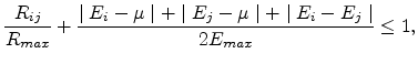 |
(1.9) |
with
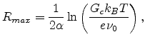 |
(1.10) |
 |
(1.11) |
 is the maximum distance between any two sites between which a
hop can occur, and
is the maximum distance between any two sites between which a
hop can occur, and  is the maximum energy that any initial or final
state can have. Thus the density of states that can be part of the percolating subnetwork is
given by
is the maximum energy that any initial or final
state can have. Thus the density of states that can be part of the percolating subnetwork is
given by
 |
(1.12) |
Since the sites in the subnetwork are linked only to sites within a range
, this criterion has the form
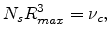 |
(1.13) |
with  being a dimensionless constant. A combination of (1.9) to (1.11) yields
Mott's law (1.8), with
being a dimensionless constant. A combination of (1.9) to (1.11) yields
Mott's law (1.8), with
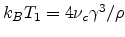 .
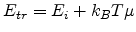
According to the Miller Abraham equation (1.1) we can roughly calculate the
nearest-neighbor distance for an upward hop from an initial site with energy
to a finial site with energy
.
According to the Miller Abraham equation (1.1) we can roughly calculate the
nearest-neighbor distance for an upward hop from an initial site with energy
to a finial site with energy
 from
the equations below [10]
from
the equations below [10]
 |
(1.14) |
Here
 is the DOS function. The hopping distance can be
calculated as
is the DOS function. The hopping distance can be
calculated as
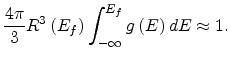
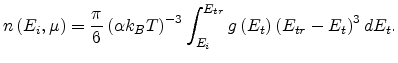
![$\displaystyle R\left(E_f\right)=\left[\frac{4\pi}{3}\int_{-\infty}^{E_f}g\left(E\right)dE\right]^{-1/3}.$](img136.png) |
(1.15) |
So the corresponding hopping rate is
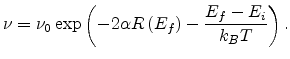 |
(1.16) |
Maximization of (1.16) over energy  gives the equation
![$\displaystyle g\left(E_f\right)\left[\int_{\infty}^{E_f}g\left(E\right)dE\right]^{-4/3}=\frac{1}{\gamma k_BT}\left(\frac{9\pi}{2}\right)^{1/3}.$](img139.png) |
(1.17) |
The finial energy that maximizes the hopping probability does not depend
on the initial energy . This particular energy is called transport
energy  [10].
[10].
Arkhipov extended this theory to the effective transport energy
[18]. In this theory, the Miller Abrahams equation is rewritten as
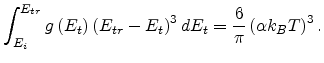
![$\displaystyle \nu=\nu_0\exp\left(-\mu\left(R_{ij}, E_i, E_j\right)\right)=\nu_0\exp\left[-2\alpha R_{ij}-\frac{\theta\left(E_j-E_i\right)}{k_BT}\right],$](img140.png) |
(1.18) |
with the hopping parameter  and the unity step function
  . The average number
 of target sites for a
starting site with energy , whose hopping parameters are not larger than
can be calculated as
of target sites for a
starting site with energy , whose hopping parameters are not larger than
can be calculated as
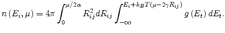 |
(1.19) |
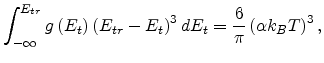
Neglecting the downward jumps and defining
 |
(1.20) |
transform (1.19) into
 |
(1.21) |
According to variable range hopping theory [19], a hop is possible if
there is at least one such hopping neighbor, i.e.  . This leads to
the following equation
. This leads to
the following equation
 |
(1.22) |
If the DOS distribution decreases with energy faster than  then the integral on the left-hand side of (1.22) depends weakly upon the
lower bound of integration for sufficiently deep starting sites, and
(1.22) is reduced to
then the integral on the left-hand side of (1.22) depends weakly upon the
lower bound of integration for sufficiently deep starting sites, and
(1.22) is reduced to
 |
(1.23) |
where is the effective transport energy.
To investigate charge transport and charge
buildup in  films, an analysis of hole transport has been presented which
is predicated on a model involving stochastic hopping transport. This
description, based on the work of Scher and Montroll [20], accounts for many
of the features of hole conduction in and has been termed the
continuous-time random walk (CTRW) model. A wide range of experimental
observation can be understood on this basis [20,21,22]. However, there has been some reticence to accept the CTRW
model completely because of observations that the apparent activation energy
for the charge collection process depends on the fraction of charge collected
[23]. This observation is at odds with the CTRW model as it has been
presented, since that model predicts universality, i.e., charge transport
curves obtained at different temperature should superimpose with a simple shift
in the time axis [24]. Although charge collection curves curves obtained at
different temperature do superimpose approximately, there is some deviation,
and this deviation is in the direction predicted by the multiple-trapping
model.
films, an analysis of hole transport has been presented which
is predicated on a model involving stochastic hopping transport. This
description, based on the work of Scher and Montroll [20], accounts for many
of the features of hole conduction in and has been termed the
continuous-time random walk (CTRW) model. A wide range of experimental
observation can be understood on this basis [20,21,22]. However, there has been some reticence to accept the CTRW
model completely because of observations that the apparent activation energy
for the charge collection process depends on the fraction of charge collected
[23]. This observation is at odds with the CTRW model as it has been
presented, since that model predicts universality, i.e., charge transport
curves obtained at different temperature should superimpose with a simple shift
in the time axis [24]. Although charge collection curves curves obtained at
different temperature do superimpose approximately, there is some deviation,
and this deviation is in the direction predicted by the multiple-trapping
model.
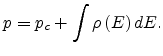
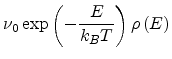
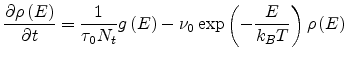
The multiple-trapping model for unipolar conduction is defined by the
following equations [12]
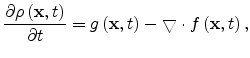 |
(1.24) |
where
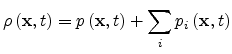 |
(1.25) |
and
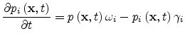 |
(1.26) |
Here
 is the local photogeneration rate,
  is the flux of mobile charge carriers,
the total carrier concentration is
is the flux of mobile charge carriers,
the total carrier concentration is
 ,
,
 is concentration of mobile carriers,
 is the carrier concentration temporarily
immobilized in the th trap,
is the carrier concentration temporarily
immobilized in the th trap,  is the capture rate by the th trap and
 is the release rate.
Later multiple trapping theory was extended for
disordered organic semiconductors as:
 |
(1.27) |
Here  is the total hole concentration,
  is the hole concentration in
extended states and
is the hole concentration in
extended states and
 is the
energy distribution of localized (immobile) holes. Since carrier trapping
does not change the total carrier concentration , the continuity equation
can be written as
is the
energy distribution of localized (immobile) holes. Since carrier trapping
does not change the total carrier concentration , the continuity equation
can be written as
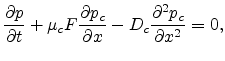 |
(1.28) |
with the mobility  and the diffusion coefficient
  . This equation assumes
two simplifications: no carrier recombination and constant electric field (no
space charge). Substituting the trapping rate
. This equation assumes
two simplifications: no carrier recombination and constant electric field (no
space charge). Substituting the trapping rate
 |
(1.29) |
and release rate
 |
(1.30) |
gives the following equation
 |
(1.31) |
In equilibrium the energy distribution of localized carriers is
established, and the function
does not depend upon time
 |
(1.32) |
Next: 1.4 Organic Light-Emitting Diodes
Up: 1. Introduction
Previous: 1.2 Organic Semiconductor Physics
Ling Li: Charge Transport in Organic Semiconductor Materials and Devices