Next: 2.4 Unified Mobility Model
Up: 2. Mobility Models for
Previous: 2.2 Carrier Concentration Dependence
Subsections
VRH theory has been applied successfully to describe the temperature dependence of
conductivity in organic materials [17,43,59]. However,
it is more difficult to obtain the experimentally
observed electric field dependence. In this section, we extend the VRH theory
to get a temperature and electric field
dependent conductivity model.
For a disordered organic semiconductor we assumed that localized
states are randomly distributed in both energy and space coordinates, and that they
form a discrete array of sites. The presented theoretical calculations are applied to explain recent
experiment. A good agreement between theory and experiment is observed.
When an electric field  exists, the transition rate of a carrier hopping from site
  to site
  is described as [60]
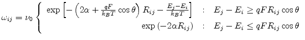 |
(2.10) |
where  is the angle
between
is the angle
between  and
and  . Assuming no correlation between the occupation probabilities of different
localized states, the current between the two sites is given by
. Assuming no correlation between the occupation probabilities of different
localized states, the current between the two sites is given by
where  and
and  are the chemical potentials of sites and , respectively [64].
To determine the conductivity of an
organic system, one can use percolation theory, regarding the system as a random
resistor network [61,62]. In the case of low electric field, the
resulting voltage drop over a single hopping distance
 is small. The conductance between sites
and can be simplified from (2.11) to the form
is small. The conductance between sites
and can be simplified from (2.11) to the form
 |
(2.11) |
Using the same derivation discussed in the previous section, we obtain as a
result the percolation criterion for an organic system as
 |
(2.12) |
with
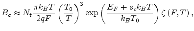
This yields the expression for the conductivity as
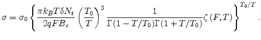 |
(2.13) |
Equation (2.13) is obtained assuming
- that the site positions are random,
- the energy barrier for the critical hop is large compared to
 ,
,
- and the charge carrier concentration is very low.
To describe the mobility, we use the mobility definition given by
[63]
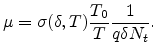 |
(2.14) |
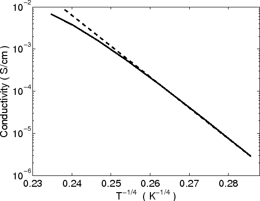
Figure 2.6:
Plot of
 versus
  at the electric field
 .
.
|
|
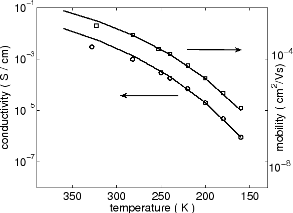
Figure 2.7:
Conductivity and mobility versus temperature for ZnPc as obtained from
the model (2.13) and (2.14) in comparison with experimental data (symbols).
|
|
Using expression (2.13), the conductivity has been calculated as a function of T at an
electric field of  V/cm, as shown in Fig 2.6. One can see
the linear dependence of conductivity on (the dashed line
is a guide to the eye). We also use the presented model to calculate the temperature and electric field
dependences of the conductivity and mobility of ZnPc (Zinc phthalocyanine). In Fig 2.7, the results
are obtained from (2.13) using
V/cm, as shown in Fig 2.6. One can see
the linear dependence of conductivity on (the dashed line
is a guide to the eye). We also use the presented model to calculate the temperature and electric field
dependences of the conductivity and mobility of ZnPc (Zinc phthalocyanine). In Fig 2.7, the results
are obtained from (2.13) using
 ,
,  and
and

 . The experimental data is from
[63].
. The experimental data is from
[63].
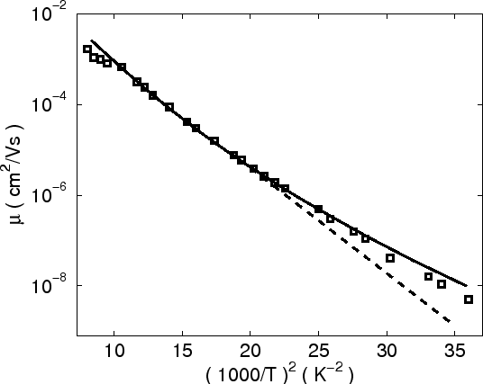
Figure 2.9:
The same data as in Fig 2.8 plotted versus  .
.
|
|
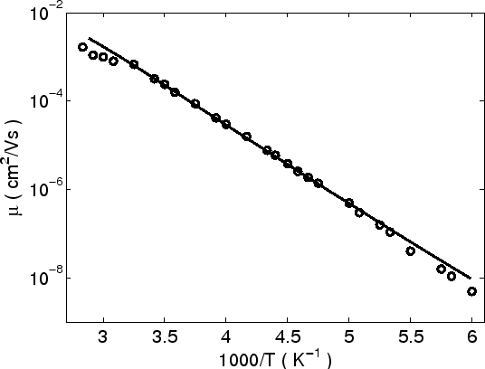
Fig 2.8 and Fig 2.9 show the mobility plotted semilogarithmically
versus  and , respectively. Symbols are TOF (time of flight)
experimental data for ZnPc from
[65] and the solid lines are the results of the analytical model. The
dashed line is to guide the eye. In both
presentations a good fit is observed. But when plotted as
and , respectively. Symbols are TOF (time of flight)
experimental data for ZnPc from
[65] and the solid lines are the results of the analytical model. The
dashed line is to guide the eye. In both
presentations a good fit is observed. But when plotted as  versus
, the slope is reduced when temperature is lower than the transition
temperature
versus
, the slope is reduced when temperature is lower than the transition
temperature
 K. This transition has also been observed by
Monte-Carlo simulation [48].
K. This transition has also been observed by
Monte-Carlo simulation [48].
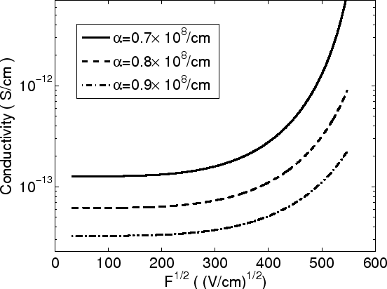
Figure 2.10:
Plot of
versus
 at
at  K.
K.
|
|
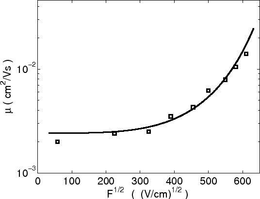
Figure 2.11:
Electric field dependence of the mobility at 290K. Symbols represent Monte Carlo
results [49], the line represents our work with parameter
 =
= K.
K.
|
|
The field dependence of the
conductivity is presented in Fig 2.10. The conductivity is approximately constant for very low fields, and
increases as we increase the field. This is the result of the fact that the field can
decrease the activation energy for forward jumps, enabling the motion of
carriers. In Fig 2.11
we also compare the mobility (2.14) to the Monte-Carlo result reported in [49].
With increasing electric field, the voltage drop over a single hopping distance
increases. If this voltage drop is of the order of or larger, the
approximate expression (2.13) for conductivity does not longer hold. The current
between the two sites depends on the chemical potential of the sites, which
in turn depends on the strength and direction of the electric field. Therefore, a
percolation model is usually adopted, assuming site-to-site hopping currents instead of
conductance [64].
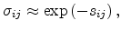
However, in this case, a conductivity model for the high electric field regime can only be
obtained after some approximations. According to percolation theory, the
critical percolation cluster of sites would comprise a current carrying
backbone with at least one site-to-site current equal to the threshold
value. Since a steady-state situation would prescribe a constant current
throughout the whole current carrying backbone, the charge will redistribute
itself along the path, thus changing the chemical potentials of sites. Hapert
omitted this rearrangement by optimization of the current with
tunneling [64]. Potentially, the redistribution of charge would change the tunneling
current, but this effect seems negligible compared to large spread  . As
a result, the conductivity between two sites is given by
. As
a result, the conductivity between two sites is given by
 |
(2.15) |
with
 |
(2.16) |
Combining (2.2), (2.8) and (2.16), the following expression for the percolation criterion is
obtained.
![$\displaystyle B_c\approx \frac{N_t}{2}\left[1+\frac{\delta}{\Gamma\left(1-T/T_0...
...mma\left(1+T/T_0\right)}\right]\int{d\bf {R_{ij}}}\theta\left(s_c-s_{ij}\right)$](img247.png) |
(2.17) |
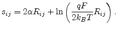
This gives the conductance as
 |
(2.18) |
where
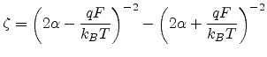
![$\displaystyle \eta=-\frac{2k_BT}{qF}\ln\left[1-\left(\frac{qF}{2k_BT}\right)^3\...
...(1+\delta/{\Gamma\left(1-T/T_0\right)\Gamma\left(1+T/T_0\right)}\right)}\right]$](img249.png) |
(2.19) |
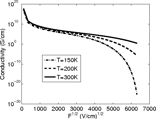
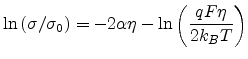
In Fig 2.12, the conductivity is presented logarimically as a function of
for high electric field . In this case, a field-saturated drift velocity, i.e.
 , is observed in accordance with the simulation work [66]
and experiment [67]. At very high fields the effective
disorder seen by a migrating carrier vanishes and backward transitions are
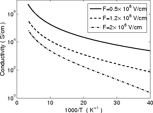
excluded [9]. The temperature dependence of conductivity at the
electric field of
, is observed in accordance with the simulation work [66]
and experiment [67]. At very high fields the effective
disorder seen by a migrating carrier vanishes and backward transitions are
excluded [9]. The temperature dependence of conductivity at the
electric field of
 V/cm is presented in
Fig 2.13. An Arrhennius-like temperature dependence
V/cm is presented in
Fig 2.13. An Arrhennius-like temperature dependence
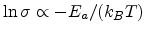 is also observed at low temperature.
Figure 2.12:
Field dependence of the conductivity at different temperatures.
|
|
Figure 2.13:
Temperature dependence of the conductivity at different electric fields.
|
|
Next: 2.4 Unified Mobility Model
Up: 2. Mobility Models for
Previous: 2.2 Carrier Concentration Dependence
Ling Li: Charge Transport in Organic Semiconductor Materials and Devices
![$\displaystyle I_{ij}=\nu_0\exp\left[-2\alpha R_{ij}-\frac{\mid E_j-E_i+qF\cos\t...
...{E_i-\mu_i}{2k_BT}\right)\cosh\left(\frac{E_j-\mu_j}{2k_BT}\right)\right]^{-1},$](img223.png)