Next: 6. Space Charge Limited
Up: 5. Charge Injection Models
Previous: 5.2 Diffusion Controlled Injection
Subsections
The steady-state injection current in an OLED is the difference between the
injection current from the electrode towards the organic semiconductor,  , and the
recombination current,
, and the
recombination current,  , from the organic semiconductor back to the electrode. The
first one is traditionally described by classical injection expressions,
either FN or RS expression. In this work and enter of a
master equation that describes the transport
at the interface by a rate equation. This model yields the injection current as a function of electric field,
temperature, energy barrier between metal and organic layer, and energetic width
of the distribution of hopping sites. Good agreement with experimental data is
found.
The system to be considered here is an energetically and positionally
random hopping system in contact with a metallic electrode. At
an arbitrary distance
, from the organic semiconductor back to the electrode. The
first one is traditionally described by classical injection expressions,
either FN or RS expression. In this work and enter of a
master equation that describes the transport
at the interface by a rate equation. This model yields the injection current as a function of electric field,
temperature, energy barrier between metal and organic layer, and energetic width
of the distribution of hopping sites. Good agreement with experimental data is
found.
The system to be considered here is an energetically and positionally
random hopping system in contact with a metallic electrode. At
an arbitrary distance  away from the metal-organic layer interface, located
at
away from the metal-organic layer interface, located
at  , the electrostatic potential is given by the sum of the
image charge potential and the applied potential described by electric field
, the electrostatic potential is given by the sum of the
image charge potential and the applied potential described by electric field  as (5.1). Since the rapid variation of potential (5.1) takes place in front of
the cathode, and
space-charge effects can be ignored altogether in the calculation of the cathode
characteristics [112,117], the field may be regarded as being nearly constant.
as (5.1). Since the rapid variation of potential (5.1) takes place in front of
the cathode, and
space-charge effects can be ignored altogether in the calculation of the cathode
characteristics [112,117], the field may be regarded as being nearly constant.
Assuming no correlations between the occupation probabilities of different
localized sates, the net electron flow between two states is
given as
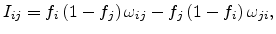 |
(5.11) |
with  denoting the occupation probability of site
  and
and
 the electron transition rate of the hopping process between the occupied state
to the empty state
the electron transition rate of the hopping process between the occupied state
to the empty state  . The probabilities (5.11) are then employed in a master
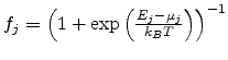
equation for describing charge transport. With the electrochemical potential
. The probabilities (5.11) are then employed in a master
equation for describing charge transport. With the electrochemical potential  at
the position of state the occupation probability is described by
a Fermi-Dirac distribution as
at
the position of state the occupation probability is described by
a Fermi-Dirac distribution as
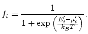 |
(5.12) |
For the metal electrode we assume a fixed electron
concentration  and a Fermi-level of zero. All injected carriers are
assumed to hop from
the metal Fermi-level. Under the effect of a constant electric field and the Coulomb field binding the carrier
with its image charge on the electrode the energy and the electrochemical potential of a localized state are given
by
and a Fermi-level of zero. All injected carriers are
assumed to hop from
the metal Fermi-level. Under the effect of a constant electric field and the Coulomb field binding the carrier
with its image charge on the electrode the energy and the electrochemical potential of a localized state are given
by
where  denotes the distance of state from the interface,
  the angle between and ,
  the barrier height, and
  the energy at state without
electric field.
According to Mott's formalism [44], the transition rate
the energy at state without
electric field.
According to Mott's formalism [44], the transition rate
 from the metal Fermi-level to state
reads as
from the metal Fermi-level to state
reads as
![$\displaystyle \omega_{j}\propto\left\{\begin{array}{r@{\quad:\quad}l}\exp\left[...
...j'\ge 0 [6pt] \exp\left(-2\alpha R_{j}\right) & E_j'\leq 0 \end{array}\right.$](img488.png) |
(5.13) |
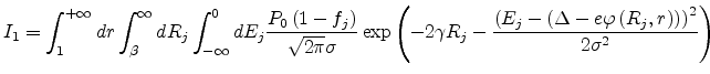
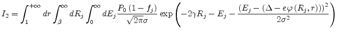
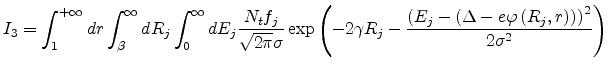
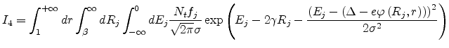
Connecting with a Gaussian DOS,
the net current across the metal-organic contact can be written as
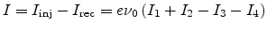 |
(5.14) |
where  is the attempt-to-jump frequency and
where
 ,
,  is the distance from the electrode to the first
hopping site in the bulk and
is the distance from the electrode to the first
hopping site in the bulk and
 .
.  and
and  describe the charge
injection from the electrode downwards and upwards, respectively.
describe the charge
injection from the electrode downwards and upwards, respectively.  and
and  describe the
backflow of charge to the electrode. The net current can be calculated by evaluating
, , and numerically.
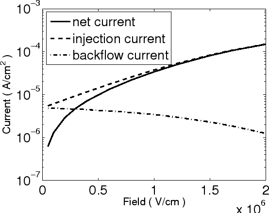
With the model presented we calculate the field dependence of the net,
injection and backflow current. The parameters are
describe the
backflow of charge to the electrode. The net current can be calculated by evaluating
, , and numerically.
With the model presented we calculate the field dependence of the net,
injection and backflow current. The parameters are
 eV,
eV,
 cm
cm ,
,  K,
K,
 =3,
=3,  nm,
nm,
 cm
cm ,
,
 eV
and
eV
and
 s. Fig 5.5 shows that with electric field the injection current
increases and the backflow current decreases, as intuitively expected. As a result, the net current increases with
electric field quickly in the low field regime.
s. Fig 5.5 shows that with electric field the injection current
increases and the backflow current decreases, as intuitively expected. As a result, the net current increases with
electric field quickly in the low field regime.
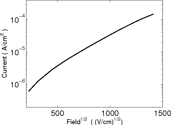
Fig 5.6 shows a
semilogarithmic plot of the current versus  with the same parameters
as used in Fig 5.5. This presentation is appropriate for testing RS behavior as
with the same parameters
as used in Fig 5.5. This presentation is appropriate for testing RS behavior as
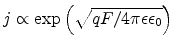 . Since the
dependence of
. Since the
dependence of  versus is not linear, a deviation from the RS
characteristics is observed.
versus is not linear, a deviation from the RS
characteristics is observed.
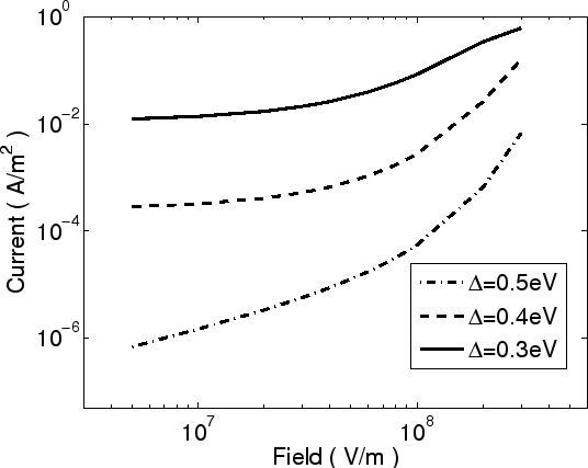
Fig 5.7 shows the current-field
characteristics for different and
 s, the other parameters are the same as in
Fig 5.5. The injection current increases with decreasing barrier height and with
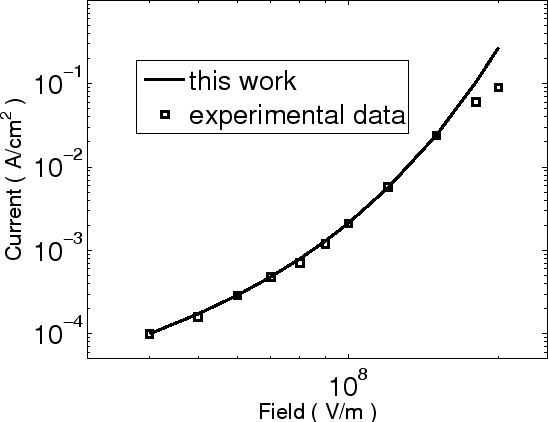
electric field. The comparison between calculation and experimental data of DASMB
sandwiched between ITO and Al electrodes [112] is given in
Fig 5.8. The parameters are
s, the other parameters are the same as in
Fig 5.5. The injection current increases with decreasing barrier height and with
electric field. The comparison between calculation and experimental data of DASMB
sandwiched between ITO and Al electrodes [112] is given in
Fig 5.8. The parameters are
 eV and
  K, the other parameters
are the same as in Fig 5.5.
The agreements is quite good at low electric fields.
The discrepancy between calculation and experimental data comes from the
resistance of the ITO contact at high electric field [112].
K, the other parameters
are the same as in Fig 5.5.
The agreements is quite good at low electric fields.
The discrepancy between calculation and experimental data comes from the
resistance of the ITO contact at high electric field [112].
Figure 5.5:
Field dependence of the net, injection, and backflow currents.
|
|
Figure 5.6:
Relation between injection current and .
|
|
Figure 5.7:
Barrier height dependence of the injection current.
|
|
Figure 5.8:
Comparison between calculation and experimental data at  .
.
|
|
Next: 6. Space Charge Limited
Up: 5. Charge Injection Models
Previous: 5.2 Diffusion Controlled Injection
Ling Li: Charge Transport in Organic Semiconductor Materials and Devices