Next: Bibliography
Up: E. Diffraction in Far
Previous: E.2 Circular Aperture
E.3 Rectangular Aperture
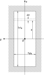
Figure E.6 shows the aperture plane with
the coordinates  and
and  .
.
Figure E.6:
Coordinate system in a rectangular aperture
 |
The transmission function is
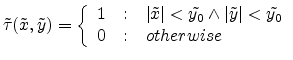 |
(E.54) |
The area of the aperture is given by
 . The
FOURIER transform can be calculated from
(E.27) and splitted into two integrals
. The
FOURIER transform can be calculated from
(E.27) and splitted into two integrals
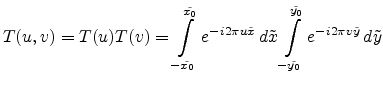 |
(E.55) |
One stripe in Figure E.6 is thereby
given by
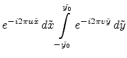 |
(E.56) |
Integration of (E.55) is simple and
straightforward
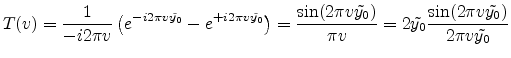 |
(E.57) |
The rightmost term can be defined as a new function
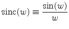 |
(E.58) |
With this substitution (E.57)
yields
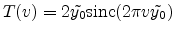 |
(E.59) |
and
 |
(E.60) |
in an analogous way.
Therefore in Point  the electric field is according to
(E.29)
the electric field is according to
(E.29)
![$\displaystyle E'(u,v) = E'(0,0)\frac{2x_0 \sinc (2\pi u\tilde{x_0})2y_0\sinc (2...
...0}\tilde{y_0}}\left[\frac{R_{00}R'_{00}}{R_0R'_0}\right]e^{i(\phi_0-\phi_{00})}$](img607.png) |
|
![$\displaystyle = E'(0,0) \sinc (2\pi u\tilde{x_0})\sinc (2\pi \tilde{y_0})\left[\frac{R_{00}R'_{00}}{R_0R'_0}\right]e^{i(\phi_0-\phi_{00})}$](img608.png) |
(E.61) |
and the intensity as the square of the electrical field is then
![$\displaystyle I'(u,v) = I'(0,0) \sinc ^2(2\pi u \tilde{x_0}) \sinc ^2(2\pi v\tilde{y_0})\left[\frac{R_{00}R'_{00}}{R_0R'_0}\right]^2$](img609.png) |
(E.62) |
For the special case of the source being located on the z-axis, the
coordinates  are zero and the coordinates
  are the following
functions of
are the following
functions of 
 and and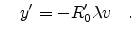 |
(E.63) |
For  and
and  (the direct beam) the coordinates are
  and according to
(E.63)
and according to
(E.63)  . The direct beam is therefore
in the z-axis and
. The direct beam is therefore
in the z-axis and
 can be written as
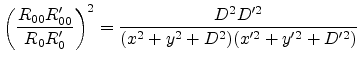
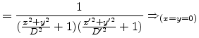
Together with (E.14) and
(E.64) the square of the fraction in
(E.62) gives
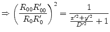
Therefore this fraction can be set to unity if
 .
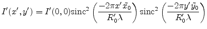
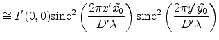
This assumption yields finally for the intensity behind a rectangular aperture
.
This assumption yields finally for the intensity behind a rectangular aperture
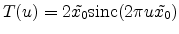
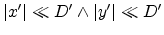
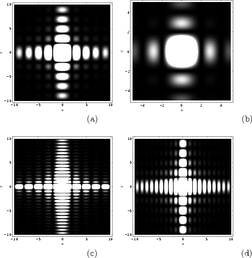
Figure E.7:
Comparison of different intensity distributions after diffraction
at a rectangular aperture (a) square aperture (b) detail of
square aperture (c) rectangular aperture with
 (d) rectangular aperture with

 |
Next: Bibliography
Up: E. Diffraction in Far
Previous: E.2 Circular Aperture
R. Minixhofer: Integrating Technology Simulation
into the Semiconductor Manufacturing Environment