Because of the large number of involved design parameters, performance improvement of QCLs requires a systematic multi-objective optimizer in conjunction with a simulation tool which has a good balance between computational speed and physical accuracy.
Various approaches such as rate equations [202,203], Monte-Carlo simulations [204], density matrix methods [205], and the non-equilibrium Green’s function formalism (NEGF) [206,207] have been developed for the simulation of QCLs.
The simplest models, based entirely on scattering and neglecting coherence effects, require a fewer number of material parameters and are generally able to predict the threshold current density but not the light-current or current-voltage characteristics [208]. Pure quantum mechanical models based on NEGF or the density matrix have been used as rigorous approaches to capture the QCL physics. The NEGF theory takes into account incoherent scattering with phonons, impurities, and rough interfaces as well as electron-electron scattering in the Hartree approximation [206]. Unfortunately, the inherently high computational costs of the full quantum mechanical models render them unfeasible for optimization purposes [206].
To study electronic transport in QCL, we employ the Pauli-master equation solved by the Monte-Carlo method [209]. In this semi-classical approach, the transport is modeled via scattering between energy states, including acoustic and optical deformation potential and polar optical electron-phonon scattering as well as alloy, inter-valley, and interface roughness scattering. Accurate results along with a relatively low computational cost render this approach as a good candidate for optimization studies.
Although quantum cascade structures (QCSs) have a long history, many aspects of the carrier transport and interaction with light field are still unclear. Very important question concerning physics of the QCSs is whether transport is coherent or incoherent. There were many discussions about the problem, and several attempts to estimate the kind of transport were successful, especially [210,211]. The answer on this question depends on conditions of QCSs operation. For example, the coherent electron transport is of interest in the non-equilibrium regime at femtosecond and picosecond time intervals. The incoherent transport is prevalent at the high excitation level in the stationary quasi-equilibrium regime. In both cases, the electronic transport influences the optical properties of the device. In this connection, the development of the theory for coherent and incoherent electron transport regimes, included many-body effects and light-matter interactions in QCS, is of actual interest. We employed the Pauli master equation [212] to model current transport through the QCL semiconductor heterostructure. Based on the experiences of a MATLAB prototype presented in [204], an optimized Monte Carlo (MC) simulator has been implemented in C++ within the Vienna-Schr¨odinger-Poisson (VSP) simulation framework [213,214].
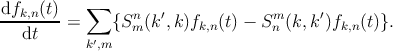
In many practical cases the steady state transport in QCLs is incoherent such that a semiclassical description can be employed [210,215]. Following this approach, a transport simulator for quantum cascade lasers based on the Pauli master equation [204] has been developed. The transport is described via scattering transitions among quasistationary basis states which are determined by numerically solving the Schr¨odinger equation. The Hamiltonian includes the band edge formed by the heterostructure. In this way, tunneling is accounted for through the delocalized eigenstates. The transport equations are derived from the Liouville von Neumann equation in the Markov limit in combination with the diagonal approximation. This means that the off-diagonal elements of the density matrix are neglected and one arrives at the Boltzmann-like Pauli master equation [216]
|
| (6.1) |
Here, m and n denote the subband indices, and k and k′ the in-plane wave vectors. The transition rate from state |k′,m⟩ to state |k,n⟩ for an interaction Hint follows from Fermi’s golden rule
 | (6.2) |
The simulator makes use of the translational invariance of the QCL structure and simulate the electron transport over a single stage only [217]. The wave function overlap between the central stage and spatially remote stages is small. It is therefore assumed that interstage scattering is limited only to the nearest neighbor stages and that interactions between basis states of remote stages can be safely neglected. The states of the whole QCL device structure are assumed to be a periodic repetition of the states of a central stage. This approach ensures charge conservation and allows imposing periodic boundary conditions on the Pauli master equation. Since transport is simulated over a central stage only, every time a carrier undergoes an interstage scattering process the electron is reinjected into the central stage with an energy changed by the voltage drop over a single period. The total current is determined by the net number of interstage transitions. The transport equations is solved using a Monte Carlo approach. Several new numerical methods are employed to reduce the computational cost of the simulation [209].
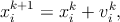
The PSO is an iterative method which initializes a number of vectors (called particles) randomly within the search space of the objective function. The set of particles is known as the swarm. Each particle represents a potential solution to the problem expressed by the objective function. During each time step the objective function is evaluated to establish the fitness of each particle using its position as input. Fitness values are used to determine which positions in the search space are better than others. Particles are then made to fly through the search space being attracted to both their personal best position as well as the best position found by the swarm so far [218]. The particles are flown through the search space by updating the position of the ith particle at time step k according to the following equation [218]:
 | (6.3) |
where xik and v ik are vectors representing the current position and velocity, respectively. Assuming vectors of dimension, the updates of the jth velocity component is governed by the following equation [219]
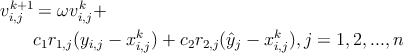 | (6.4) |
where 0 < ω < 1 is an inertia weight determining how much of the particle’s previous velocity is preserved, c1 and c2 are two positive acceleration constants, r1,j and r2,j are two uniform random sequences sampled from U(0,l), yi is the personal best position found by the ith particle and ŷ is the best position found by the entire swarm so far. The following relation should hold in order for the PSO to converge [218]:
 | (6.5) |
However, the standard PSO is not guaranteed to converge on a local extremum, but most of the recent PSO algorithms converge to the global optimum.
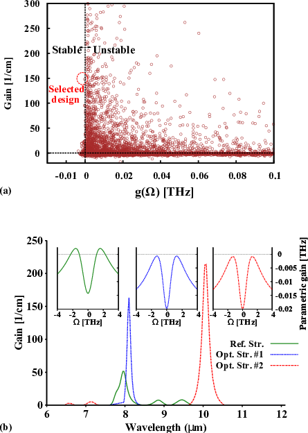
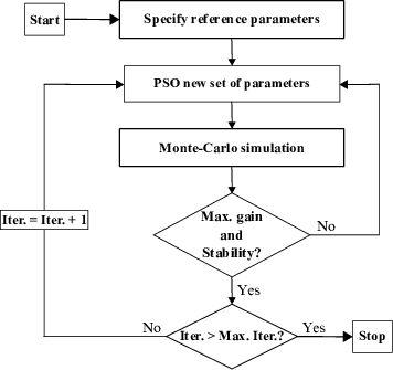
Employing a Pauli master equation-based description of electronic transport in QCLs along with the multi-objective PSO strategy, a framework is developed for maximizing laser gain with simultaneous desirable instability operation. In this framework one starts from a reference design. In the next iterations the well and barrier thicknesses and the applied electric field are modified until maximum gain and laser operation below the instability threshold are achieved. The analytical linear stability model introduced in Ref. [126] is employed to analyze the instability threshold of the studied QCL. In this model, the criteria for the RNGH instability is expressed in terms of the parametric gain g(Ω) as a function of the resonance frequency Ω
![g(Ω ) = - c-Re [l0--(ΩT1--+-i)ΩT2----2(pf---1)--+
2n (ΩT1 + i)(ΩT2 + i) - (pf - 1)
γℏ2(p - 1)(ΩT + i)(3 ΩT + 2i) - 4(p - 1)
---2-f---------1---------2------------f-----],
μ T1T2 (ΩT1 + i)(ΩT2 + i) - (pf - 1)](diss169x.png) | (6.6) |
where pf is the pumping factor, T1 is the gain recovery time, T2 is the dephasing time, l0 is the linear cavity loss, μ is the matrix element of the lasing transition, and γ is the SA coefficient. The derivation of Eq.6.6 is presented in detail in Appendix C. Based on this analysis, each mode which is identified by the resonance frequency Ω, is stable if the parametric gain is negative, otherwise it is unstable. At each iteration of the optimization loop, for a set of geometrical parameters and the applied electric field, the parameters T1 and μ are extracted and the parametric gain (Eq. 6.6) is evaluated. The parameter T2, dephasing time, can be approximated by T1∕10 as mentioned in [220]. If the stability condition is not satisfied, a new set of parameters is selected for the next iteration. The flow chart of the developed framework is described in Fig. 6.1.