In the following, the particle flux equation is derived, whereby the starting
point is Boltzmann's equation with a general vector-valued weight
 in
the form of equation (3.30). For the flux equations, the time derivative
(first term in (3.30)) can be safely neglected, since the relaxation
time is in the order of picoseconds, which ensures quasi-stationary behavior
even for today's fastest signals [87]. This means that a transient
signal must only change as fast as the carriers are available to follow into a
new equilibrium state.
in
the form of equation (3.30). For the flux equations, the time derivative
(first term in (3.30)) can be safely neglected, since the relaxation
time is in the order of picoseconds, which ensures quasi-stationary behavior
even for today's fastest signals [87]. This means that a transient
signal must only change as fast as the carriers are available to follow into a
new equilibrium state.
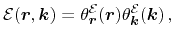
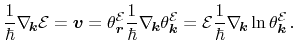
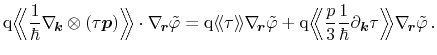
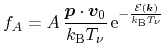
Inserting
 as
into (3.30) delivers the particle
current equation in its original form which serves as a basis for further
derivations
as
into (3.30) delivers the particle
current equation in its original form which serves as a basis for further
derivations
 |
(3.38) |
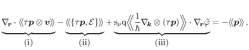
The single contributions to the left side can be identified as a diffusion term
(i)
and two drift terms
(ii)
and
(iii)
, whereby the latter one is
caused by external electric fields
(iii)
. In the sequel, these terms are
subject to several simplifications caused by assumptions on the distribution
function, the band structure, and the relaxation time.
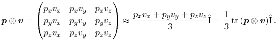
Equation (3.38) contains statistical averages of tensor-valued
quantities, which are subject to closer investigation in the following. With
the assumption of an almost isotropic distribution function, the non-diagonal
elements of the tensors are negligible. For a hot, slowly drifting electron
gas, such as discussed in Sections 3.4 and 3.5.1, the
influence of the displacement on the averages of even weights, such as
energy-like tensors is negligible [84]. Thus, each of the terms can
be represented by proper scalar quantities, which are expressed using traces of
the corresponding tensor-valued transport parameters. For example,
 can be estimated using
 |
(3.39) |
Monte-Carlo simulations indicate the validity of this approximation. It
turned out that for the case sketched above, the non-diagonal elements are
about five magnitudes smaller than the diagonal elements. In low field cases,
the assumption of isotropy is fulfilled very well for the materials taken into
account in this work.
In order to incorporate the band structure in an analytical way, assumptions on
the dispersion relation as discussed in Section 3.3 have to be
made. In order to obtain a mathematically convenient formulation, a product
ansatz for the kinetic energy separating the dependencies on
 and
and
 is
performed
is
performed
 |
(3.40) |
which will be expressed by parabolic bands later on in this derivation. As a
direct consequence, the energy's gradients in
- and
-space read
 |
|
|
(3.41) |
 |
|
|
(3.42) |
It is useful to introduce a non-parabolicity factor
 which becomes
 for parabolic bands. Thus, the velocity reads
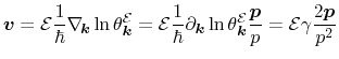 with with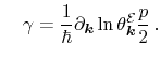 |
(3.43) |
In the following, the three parts of equation (3.38) indicated by the
horizontal braces are sequentially treated. Applying
Eqs. (3.39) and (3.43) to equation (3.38), part (i), one obtains
 |
(3.44) |
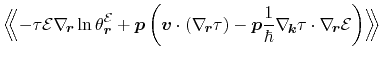
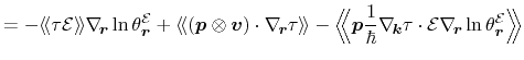
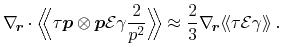
For the second part of equation (3.38), the Poisson bracket has to be
expanded using (A.10) as well as the definitions for the Poisson bracket,
equations (A.1) and (A.6)
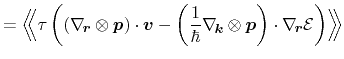
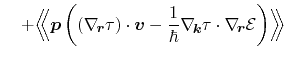
The first term vanishes due to the momentum being orthogonal to the space
vector, and finally the approximation for tensor valued quantities (3.39)
and the application of identity (B.5) leads to
Part (iii) of equation (3.38) has to be converted using identity
(B.4) before the trace approximation can be performed, which leads to
 |
(3.47) |
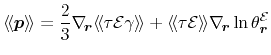
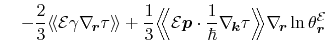
Assembling the terms (i) - (iii) again, the isotropic particle current
equation with a product ansatz used on the kinetic energy
 is obtained
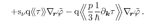
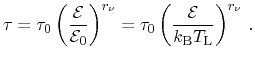
In order to obtain a closed formulation, the relaxation time has to be
parametrized with macroscopic quantities available in the equation system.
Thus, a power-law approximation is introduced as discussed in
Section 3.5.4. The according reference energy
 refers to the
energy in local thermal equilibrium with the lattice and thus incorporates the
lattice temperature.
refers to the
energy in local thermal equilibrium with the lattice and thus incorporates the
lattice temperature.
 is expressed as
 |
(3.49) |
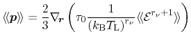
Inserting (3.49) to (3.48) yields
In order to close the equation system, a heated, displaced Maxwellian in the
diffusion approximation (3.18) is assumed. This
approximation is justified by the comparably low drift velocities in
thermoelectric devices. Furthermore, parabolic bands (3.13) are
introduced
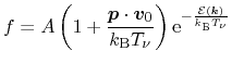 and and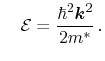 |
(3.51) |
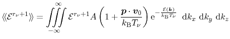
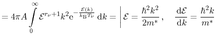
With these assumptions, the average in (i) is first transformed to polar
coordinates and furthermore to an integral in
-space and the gamma
function can be identified. The integral over the odd term of the distribution
function
 |
(3.52) |
vanishes, since the product of an even and an odd function results in
an odd function
The integral for the carrier density is derived analogously, and yields
 |
(3.54) |
whereby the identity
 has been
applied. The carrier concentration is introduced to normalize (3.50).
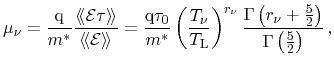
Finally, the carrier mobility is obtained from a coefficient comparison for the
homogeneous case as [73]
has been
applied. The carrier concentration is introduced to normalize (3.50).
Finally, the carrier mobility is obtained from a coefficient comparison for the
homogeneous case as [73]
 |
(3.55) |
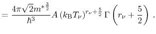
for a heated, displaced Maxwellian. Inserting equations (3.54) and (3.55) to
(3.53), part (i) becomes
 |
(3.56) |
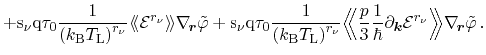
Parts (ii) and (iii) can be treated as described above. The gradient in
the second average has to be expanded resulting in the sum of two expressions,
a
 and a
and a
 term. The average needed for the
expressions of part (iii) can be derived analogously to (3.53) and
results in
term. The average needed for the
expressions of part (iii) can be derived analogously to (3.53) and
results in
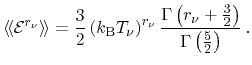 |
(3.57) |
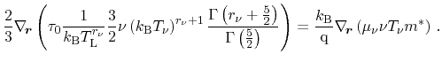
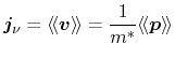
Assembling the three parts and inserting the definition of the particle flux
 |
(3.58) |
results in the final isotropic particle flux equation obtained using a
power-law approximation for the microscopic relaxation time, parabolic bands
and a heated, displaced Maxwellian
 |
(3.59) |
An alternative formulation of the current equation is obtained by combining the
gradients of the carrier concentration
 and the effective mass
  to the
chemical potential which itself is summed up with the electrostatic potential
to the
chemical potential which itself is summed up with the electrostatic potential
 to the electrochemical potential
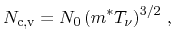
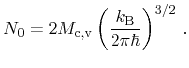
 . Therefore, the effective
density of states is introduced
[89], which is proportional to
and
. Therefore, the effective
density of states is introduced
[89], which is proportional to
and

 |
(3.60) |
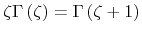
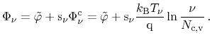
where
 reads for a Maxwellian distribution function
 |
(3.61) |
The chemical potential
 and the electrochemical potential
are
introduced as
and the electrochemical potential
are
introduced as
 |
(3.62) |
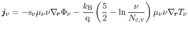
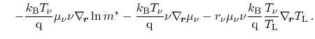
Applying Eqs. (3.60) and (3.62) to the particle current (3.59) yields
 |
|
|
(3.63) |
 |
|
|
|
M. Wagner: Simulation of Thermoelectric Devices