5.3.2 Effective Masses, Density of States, Intrinsic Carrier Density

While the effective masses for each the first conduction and valence band of lead telluride have been studied quite well in literature, only very uncertain information is available for the second valence band. Both the valence and the conduction band feature a strong anisotropy with material composition dependent values of $10-14$ [260,188]. Values based on both measurements as well as band structure calculations of the low temperature effective mass for the first conduction and valence band, respectively are collected in Table 5.8.

Table 5.8: Low temperature effective masses for the first conduction and valence band in lead telluride.

Electrons		Holes
$m_l$	$m_t$	$m_l$	$m_t$	Ref.
0.24	0.024	0.31	0.022	meas. [194]
0.238	0.031	0.426	0.034	calc. [241]
0.274	0.043			meas. [266]
		0.165	0.030	meas. [267]
0.24	0.022			meas. [199]
0.23	0.022			calc. [199]

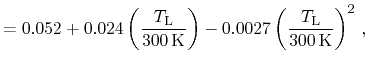
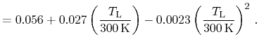
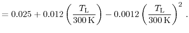
The temperature dependence of the effective masses is commonly expressed by quadratic polynomials [268]. According coefficients have been identified based on temperature dependent data in [188]. Expressions for the longitudinal and transversal effective masses for each the first conduction and valence bands in pure lead telluride read

$$\ensuremath{\ensuremath{m^*_\ensuremath{\mathrm{c,l}}}} = 0.25 + 0.11 \ensuremath{\left(\ensuremath{\frac{\ensuremath{T_{... ...\frac{\ensuremath{T_{\mathrm{L}}}}}{300\,\ensuremath{\mathrm{K}}}\right)}^2 \,,$$ (5.26)

$$\ensuremath{\ensuremath{m^*_\ensuremath{\mathrm{c,t}}}} = 0.024 + 0.0112 \ensuremath{\left(\ensuremath{\frac{\ensuremath{... ...\frac{\ensuremath{T_{\mathrm{L}}}}}{300\,\ensuremath{\mathrm{K}}}\right)}^2 \,,$$ (5.27)

$$\ensuremath{\ensuremath{m^*_\ensuremath{\mathrm{v,l}}}} = 0.286 + 0.142 \ensuremath{\left(\ensuremath{\frac{\ensuremath{T... ...\frac{\ensuremath{T_{\mathrm{L}}}}}{300\,\ensuremath{\mathrm{K}}}\right)}^2 \,,$$ (5.28)

$$\ensuremath{\ensuremath{m^*_\ensuremath{\mathrm{v,t}}}} = 0.025 + 0.012 \ensuremath{\left(\ensuremath{\frac{\ensuremath{T... ...\frac{\ensuremath{T_{\mathrm{L}}}}}{300\,\ensuremath{\mathrm{K}}}\right)}^2 \,.$$ (5.29)

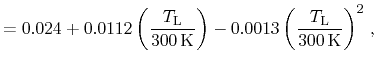
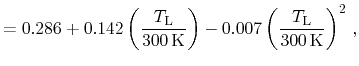
The according temperature dependencies of the density-of-states masses derived by

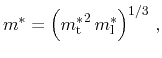$$m^*= \left( \ensuremath{{m^*_\ensuremath{\mathrm{t}}}}^2 \,\ensuremath{m^*_\ensuremath{\mathrm{l}}}\right)^{1/3} \,,$$ (5.30)

have been identified as

$$\ensuremath{m^*_\ensuremath{\mathrm{c}}} = 0.052 + 0.024 \ensuremath{\left(\ensuremath{\frac{\ensuremath{T... ...{\frac{\ensuremath{T_{\mathrm{L}}}}}{300\,\ensuremath{\mathrm{K}}}\right)}^2\,,$$ (5.31)

$$\ensuremath{m^*_\ensuremath{\mathrm{v}}} = 0.056 + 0.027 \ensuremath{\left(\ensuremath{\frac{\ensuremath{T... ...{\frac{\ensuremath{T_{\mathrm{L}}}}}{300\,\ensuremath{\mathrm{K}}}\right)}^2\,.$$ (5.32)

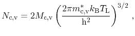
Since the extrema of both the first conduction and valence band are located at the L point, the number of equivalent valleys within the Brillouin zone $\ensuremath{M_\mathrm{c,v}}$ is 4. Thus, the effective density of states including spin-degeneracy can be expressed by [269]

$$\ensuremath{N_\mathrm{c,v}}= 2 \ensuremath{M_\mathrm{c,v}}\left( ... ...rm{B}}\ensuremath{T_{\mathrm{L}}}}{\ensuremath{\mathrm{h}}^2} \right)^{3/2} \,,$$ (5.33)

and the intrinsic carrier concentration is derived as

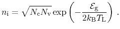$$\ensuremath{n_\mathrm{i}}= \sqrt{\ensuremath{N_\mathrm{c}}\ensure... ...mathrm{g}}}}}{2k_\ensuremath{\mathrm{B}}\ensuremath{T_{\mathrm{L}}}}\right) \,.$$ (5.34)

Figure 5.10: Temperature dependence of the effective density of states as well as the intrinsic carrier concentration in lead telluride.

Expressions for the material composition and temperature dependent effective masses have been given by Preier [260] and Akimov [202]. While both give expressions with respect to the temperature and material composition dependent band gap, the latter does not differ between the valence and conduction band and provides a constant anisotropy ratio between the transversal and longitudinal effective masses. His expressions for the relative carrier masses read

$$\ensuremath{m^*_\ensuremath{\mathrm{t}}}(x,\ensuremath{T}) = 0.16 \,\ensuremath{\ensuremath{\mathcal{E}}_{\ensuremath{\mathrm{g}}}}(x,\ensuremath{T})$$ (5.35)

$$\ensuremath{m^*_\ensuremath{\mathrm{l}}}(x,\ensuremath{T}) = 10.5 \,\ensuremath{m^*_\ensuremath{\mathrm{t}}}(x,\ensuremath{T}) \,.$$ (5.36)

Preier differs between the according values of the valence and conduction band and implies a material composition dependent anisotropy ratio

$$\ensuremath{m^*_\ensuremath{\mathrm{c,t}}} = \left( 30.58 \frac{\ensuremath{\ensuremath{\mathcal{E}}_{\ensur... ...cal{E}}_{\ensuremath{\mathrm{g}}}}(x,\ensuremath{T})} + 14.29 \right) ^{-1} \,,$$ (5.37)

$$\ensuremath{m^*_\ensuremath{\mathrm{v,t}}} = \left( 30.58 \frac{\ensuremath{\ensuremath{\mathcal{E}}_{\ensur... ...cal{E}}_{\ensuremath{\mathrm{g}}}}(x,\ensuremath{T})} + 10.00 \right) ^{-1} \,,$$ (5.38)

$$\ensuremath{m^*_\ensuremath{\mathrm{c,l}}} = \left( \frac{30.58}{10.25 + 6.56 x} \frac{\ensuremath{\ensurema... ...hcal{E}}_{\ensuremath{\mathrm{g}}}}(x,\ensuremath{T})} + 2.42 \right) ^{-1} \,,$$ (5.39)

$$\ensuremath{m^*_\ensuremath{\mathrm{v,l}}} = \left( \frac{30.58}{10.25 + 6.56 x} \frac{\ensuremath{\ensurema... ...hcal{E}}_{\ensuremath{\mathrm{g}}}}(x,\ensuremath{T})} + 1.52 \right) ^{-1} \,.$$ (5.40)

M. Wagner: Simulation of Thermoelectric Devices