The weighted residual method is demonstrated for the scalar function ![]() and
can be applied analogously to the vector one
and
can be applied analogously to the vector one ![]() .
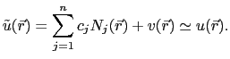
Usually the unknown function
.
Usually the unknown function ![]() of (3.1) cannot be found analytically,
therefore, it is approximated by
of (3.1) cannot be found analytically,
therefore, it is approximated by
In (3.5)
![]() is a known function which fulfills
exactly the Dirichlet boundary condition on
is a known function which fulfills
exactly the Dirichlet boundary condition on
![]()
The basis (also called form or shape) functions
![]() build a set
of linear independent known functions which vanish on the Dirichlet
boundary
build a set
of linear independent known functions which vanish on the Dirichlet
boundary
![]() . Thus (3.6) is satisfied for
each arbitrary set of coefficients
. Thus (3.6) is satisfied for
each arbitrary set of coefficients
![]() . The coefficients
. The coefficients
![]() must be determined in such a way that the function
must be determined in such a way that the function ![]() approximates the solution of (3.1) as exactly as possible.
The basis functions should be formulated in such way that each
solution can be approximated with arbitrary accuracy,
if a sufficiently large number of basis functions is used.
After substitution of
approximates the solution of (3.1) as exactly as possible.
The basis functions should be formulated in such way that each
solution can be approximated with arbitrary accuracy,
if a sufficiently large number of basis functions is used.
After substitution of
![]() for
for ![]() in (3.1) a nonzero residual is
obtained in general
in (3.1) a nonzero residual is
obtained in general
To find a good approximation ![]() for
for ![]() it is required to minimize
the residual (3.7). The weighted residual method finds
the unknown coefficients
it is required to minimize
the residual (3.7). The weighted residual method finds
the unknown coefficients ![]() by weighting the residual (3.7).
This is performed by choosing a set of linear independent weighting (called test or trial)
functions
by weighting the residual (3.7).
This is performed by choosing a set of linear independent weighting (called test or trial)
functions
![]() ,
, ![]() and by enforcing the condition
and by enforcing the condition
Insertion of (3.7) in (3.8) gives
which leads to the following expression to obtain the coefficients ![]()
Since
![]() is a
linear differential operator (3.10) becomes
is a
linear differential operator (3.10) becomes
which corresponds to a linear equation system
The Matrix ![]() and the right hand side vector
and the right hand side vector ![]() are given by the expressions
are given by the expressions
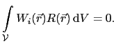
![$\displaystyle \int_{\mathcal{V}}W_i(\vec{r})\left\{\mathcal{L}\left[\tilde{u}(\vec{r})\right] - f(\vec{r})\right\} \mathrm{d}V = 0, i\in[1;n],$](img54.gif)
![$\displaystyle \int_{\mathcal{V}}W_i(\vec{r})\left\{\mathcal{L}\left[\sum_{j=1}^...
...c{r}) + v(\vec{r})\right] - f(\vec{r})\right\} \mathrm{d}V = 0, i\in[1;n].$](img55.gif)
![$\displaystyle c_j\sum_{j=1}^{n}\int_{\mathcal{V}}W_i(\vec{r})\mathcal{L}\left[N...
...c{r}) - \mathcal{L}\left[v(\vec{r})\right]\right\} \mathrm{d}V, i\in[1;n],$](img56.gif)
![\begin{displaymath}\begin{split}K_{ij} & = \int_{\mathcal{V}}W_i(\vec{r})\mathca...
...t]\right\} \mathrm{d}V, i\in[1;n], j\in[1;n]. \end{split}\end{displaymath}](img60.gif)