A. Integral Domain Transformation

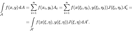
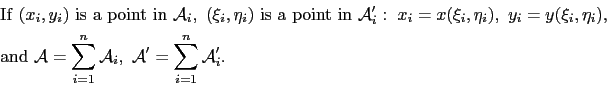
It has been shown that the barycentric coordinates transform each triangular and tetrahedron element in the unit triangle and tetrahedron, respectively. (Refer to Fig. <4.3> and Fig. <4.8>.) This is used for the analytical calculation of the arising integral terms, when the element matrices are assembled.

Figure A.1: Two-dimensional domain transformation.

The two-dimensional domain $\mathcal{A}^{\prime}$ is transformed to $\mathcal{A}$ by the expressions

$$\begin{split}x & = x(\xi, \eta) y & = y(\xi, \eta). \end{split}$$ (A.1)

$$\begin{split}& \mathrm{If} (x_i,y_i) \mathrm{is a point ... ...l{A}^{\prime} = \sum_{i=1}^n\mathcal{A}_i^{\prime}. \end{split}$$

$$\begin{split}& E^{\prime}F^{\prime}G^{\prime}H^{\prime} \righ... ...+h,\eta+k) ), H( x(\xi,\eta+k),y(\xi,\eta+k) ). \end{split}$$ (A.2)

The area $A_i$ of the $i$ -th element $EFGH$ is approximately related by the vector product

$$\vec{EF} \left\{ \begin{array}{l} x(\xi + h,\eta) - x(\xi,\eta) =... ...,\eta) - y(\xi,\eta) = y_{\xi}(\tilde{\tilde{\xi}},\eta) h \end{array} \right.$$ (A.3)

and

$$\vec{EH} \left\{ \begin{array}{l} x(\xi,\eta + k) - x(\xi,\eta) =... ...+ k) - y(\xi,\eta) = y_{\eta}(\xi,\tilde{\tilde{\eta}}) k \end{array} \right.,$$ (A.4)

where

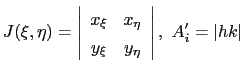
$$\tilde{\xi}\in[\xi;\xi+h], \tilde{\tilde{\xi}}\in[\xi;\xi+h], \tilde{\eta}\in[\eta;\eta+k], \tilde{\tilde{\eta}}\in[\eta;\eta+k].$$ (A.5)

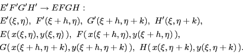
For sufficiently small $h$ and $k$ the face $A_i$ is expressed as

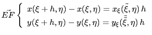
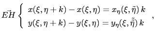
$$\begin{split}A_i & = \vert\vec{EF}\times\vec{EH}\vert = [x_{\... ...xi,\eta)]\vert hk\vert = J(\xi, \eta) A_i^{\prime} \end{split}$$ (A.6)

with

$$J(\xi, \eta) = \left\vert \begin{array}{cc} x_{\xi} & x_{\eta} y_{\xi} & y_{\eta} \end{array} \right\vert, A_i^{\prime} = \vert hk\vert$$ (A.7)

and an integral is given by the Riemann sum

$$\begin{split}\int_{\mathcal{A}}f(x,y) \mathrm{d}A & = \sum_{... ...eta),y(\xi,\eta))J(\xi,\eta) \mathrm{d}A^{\prime}. \end{split}$$ (A.8)

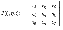
Analogously the transformation for the three-dimensional case can be expressed by:

$$\int_{\mathcal{A}}f(x,y,z) \mathrm{d}A = \int_{\mathcal{A^{\prim... ...ta),y(\xi,\eta,\zeta),z(\xi,\eta,\zeta))J(\xi,\eta,\zeta) \mathrm{d}A^{\prime}$$ (A.9)

with

$$J(\xi, \eta, \zeta) = \left\vert \begin{array}{ccc} x_{\xi} & x_{... ...y_{\eta} & y_{\zeta} z_{\xi} & z_{\eta} & z_{\zeta} \end{array} \right\vert.$$ (A.10)