4.1.1 Galerkin's Method

Multiplying (4.1) by a function $v(\vec r)$, which is called test or trial function, and integrating over the simulation domain gives the variational formulation

$$\int_{\symDomain} v(\vec r) L[u(\vec r)] d\symDomain = \int_{\symDomain} v(\vec r) f(\vec r) d\symDomain.$$ (4.2)

Using the notation

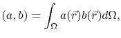$$\left(a,b\right) = \int_{\symDomain} a(\vec r)b(\vec r)d\symDomain,$$ (4.3)

(4.2) can be written as

$$\left(L[u], v\right) = \left(f, v\right).$$ (4.4)

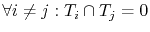
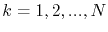
In order to obtain the corresponding discrete problem, the simulation domain, , is divided in a set of $m$ elements, $T_1, T_2,..., T_m$, which do not overlap, i.e. $\forall i\neq j: T_i\cap T_j = 0$. The mesh obtained by such a domain discretization is represented by

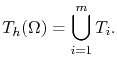$$T_h(\symDomain)=\bigcup_{i=1}^{m}T_i.$$ (4.5)

Further, one defines a set $P$ of grid points, also called nodes, with each point $p_k \in P$ being described by a unique global index $k=1,2,...,N$, where $N$ is the total number of grid points in the mesh.

The approximate solution, $u_h(\vec r)$, for the unknown function, $u(\vec r)$, is given by [152]

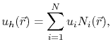$$u_h(\vec r) = \sum_{i=1}^{N} u_iN_i(\vec r),$$ (4.6)

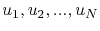
where $N_i(\vec r)$ are the so-called basis (or shape) functions. The approximate solution of (4.4) is determined by the coefficients $u_i$, which represent the value of the unknown function at the node $i$. At the node $i$, where the point is given by the coordinates $\vec r_i$, the basis functions must satisfy the condition

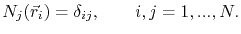$$N_j(\vec r_i) = \symKronecker,\qquad i,j=1,...,N.$$ (4.7)

Typically, the basis functions are chosen to be low order polynomials.

Substituting (4.6) in (4.4), and choosing $v=N_j(\vec r)$ one obtains

$$\left(L[\sum_{i=1}^{N} u_iN_i], N_j\right) = \left(f, N_j\right), \qquad j=1,...,N,$$ (4.8)

and since $L[\cdot]$ is a linear operator and the coefficients $u_i$ are constants one can write

$$\sum_{i=1}^{N}u_i\left(L[N_i], N_j\right) = \left(f, N_j\right), \qquad j=1,...,N.$$ (4.9)

Equation (4.9) is, in fact, a linear system of $N$ equations with $N$ unknowns, $u_1, u_2, ..., u_N$. Thus, it can be written in matrix notation as

$$\mathbf{A} \mathbf{x} = \mathbf{b},$$ (4.10)

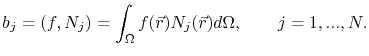
where $\mathbf{A} = (a_{ij})$ is called stiffness matrix, given by the elements

$$a_{ij} = \left(L[N_i], N_j\right) = \int_{\symDomain} L[N_i(\vec r)] N_j(\vec r) d\symDomain,\qquad i,j=1,...,N,$$ (4.11)

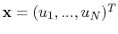$\mathbf{x} = (u_1,...,u_N)^T$ is the vector of unknown coefficients, and 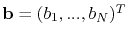$\mathbf{b} = (b_1,...,b_N)^T$ is the load vector, given by

$$b_{j} = \left(f, N_j\right) = \int_{\symDomain} f(\vec r) N_j(\vec r) d\symDomain, \qquad j=1,...,N.$$ (4.12)