Consider the simple model of Shatzkes and Lloyd, expressed by the equation (2.13).
Given a finite line of length ![]() , with blocking boundary conditions at both ends of the line, that is
, with blocking boundary conditions at both ends of the line, that is
In order to compare the numerical implementation with this analytical solution, it is set ![]() in (3.75) and
in (3.75) and
![]() in (3.74).
This makes the proposed model equivalent to equation (2.13) by removing the generation/recombination term and also neglecting the mechanical stress effects.
Figure 5.1 shows the vacancy distribution next to the blocking boundary at
in (3.74).
This makes the proposed model equivalent to equation (2.13) by removing the generation/recombination term and also neglecting the mechanical stress effects.
Figure 5.1 shows the vacancy distribution next to the blocking boundary at ![]() of a simple copper line of length
of a simple copper line of length
![]()
![]() m after a time
m after a time ![]() h, obtained from a numerical simulation.
h, obtained from a numerical simulation.
The current flows from left to right, so that vacancy accumulates at the cathode end of the line. At the same time, vacancy depletion takes place at the anode side at ![]() .
This can be seen by the vacancy concentration at the center of the line along the
.
This can be seen by the vacancy concentration at the center of the line along the ![]() direction, as shown in Figure 5.2 for different time periods.
The curve for
direction, as shown in Figure 5.2 for different time periods.
The curve for ![]() s shows the vacancy concentration distribution after the steady state is already reached.
The symbols correspond to the numerical simulation results, while the solid lines correspond to the analytical solution given in (5.2).
It should be pointed out that the agreement between the numerical and the analytical solution is excellent.
s shows the vacancy concentration distribution after the steady state is already reached.
The symbols correspond to the numerical simulation results, while the solid lines correspond to the analytical solution given in (5.2).
It should be pointed out that the agreement between the numerical and the analytical solution is excellent.
![\includegraphics[width=0.85\linewidth]{chapter_applications/Figures/SL_Cv_x.eps}](img675.png)
|
The accumulation of vacancies at the cathode and depletion at the anode creates a gradient of vacancy concentration along the line, which counters the electromigration flux.
Once the vacancy gradient produces a back flux that equals the electromigration flux, the steady state condition is reached.
The vacancy build-up with time at the boundary ![]() is shown in Figure 5.3.
The simulation results are presented for three values of current density,
is shown in Figure 5.3.
The simulation results are presented for three values of current density,
![]() , 2.0, and 5.0 MA/cm
, 2.0, and 5.0 MA/cm![]() .
The increase of current density is accompanied by the increase of the electromigration flux, which leads to a higher vacancy concentration at the cathode end of the line.
It is interesting to note that the time to reach the steady state lies in the order of minutes. After about 10 min the vacancy concentration already saturates.
As it will be shown later, this is a major shortcoming of this model.
Figure 5.3 shows that an excellent agreement between the numerical and the analytical solution is again observed.
.
The increase of current density is accompanied by the increase of the electromigration flux, which leads to a higher vacancy concentration at the cathode end of the line.
It is interesting to note that the time to reach the steady state lies in the order of minutes. After about 10 min the vacancy concentration already saturates.
As it will be shown later, this is a major shortcoming of this model.
Figure 5.3 shows that an excellent agreement between the numerical and the analytical solution is again observed.
Consider now the intersection of two metal grains forming a grain boundary, as shown in Figure 5.4.
The model of Rosenberg and Ohring, given by equation (2.21), is used to analyze the vacancy supersaturation that can develop at such a grain boundary.
The magnitude of vacancy supersaturation at the grain boundary is a function of the transport characteristics of both grains. Thus, depending on the difference of the diffusion coefficients in each grain, or on the available paths for atomic transport, different supersaturation values are expected.
![\includegraphics[width=0.85\linewidth]{chapter_applications/Figures/SL_Cv_t.eps}](img677.png)
|
![\includegraphics[width=0.90\linewidth]{chapter_applications/Figures/RO_struct.eps}](img678.png)
|
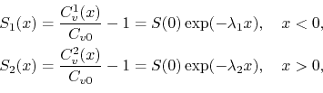
At steady state (
![]() ) both, the vacancy concentration and the flux are continuous along the grain boundary interface,
) both, the vacancy concentration and the flux are continuous along the grain boundary interface,
It is assumed that the diffusion coefficient in each grain is different, so that
![]() eV is set for the left grain, and
eV is set for the left grain, and
![]() eV is set for the right grain of the line. The other paremeters are considered to be the same for both grains.
The electric current flows from the left to the right grain, and since the activation energy for diffusion is smaller in the first grain, vacancies arrive at the grain boundary at a higher rate than they leave. As a result, vacancy accumulation takes place at the grain boundary, as shown in Figure 5.5.
eV is set for the right grain of the line. The other paremeters are considered to be the same for both grains.
The electric current flows from the left to the right grain, and since the activation energy for diffusion is smaller in the first grain, vacancies arrive at the grain boundary at a higher rate than they leave. As a result, vacancy accumulation takes place at the grain boundary, as shown in Figure 5.5.
![\includegraphics[width=0.90\linewidth]{chapter_applications/Figures/RO_Cv.eps}](img687.png)
|
The vacancy supersaturation along the grains for different vacancy relaxation times is shown in Figure 5.6. One can see that the vacancy concentration profile in each grain is quite different. The bigger diffusion coefficient leads to a smaller concentration gradient in the left grain. In turn, the smaller diffusivity in the right grain leads to a larger concentration gradient near the grain boundary. The comparison between the numerical simulations and the analytical solution, given by equation (5.8), is remarkably good.
An important observation is that the supersaturation significantly decreases as the vacancy relaxation time decreases. Furthermore, the maximum supersaturation is rather small, even for longer vacancy relaxation times.
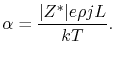
This means that the maximum supersaturation is significantly dependent on
![]() , that is, it is significantly dependent on the effectiveness of the vacancy sink/source. As a consequence, a high vacancy supersaturation cannot be obtained near vacancy sinks, since vacancies are annihilated as soon as the local vacancy concentration becomes higher than its equilibrium value.
, that is, it is significantly dependent on the effectiveness of the vacancy sink/source. As a consequence, a high vacancy supersaturation cannot be obtained near vacancy sinks, since vacancies are annihilated as soon as the local vacancy concentration becomes higher than its equilibrium value.
The time development of the vacancy supersaturation at the grain boundary obtained from the numerical simulations is presented in Figure 5.7. Besides the aforementioned strong influence on the supersaturation magnitude, the vacancy relaxation time has a significant impact on the time to reach the steady state condition. Here again, the shorter the relaxation time is, the faster vacancy annihilation or generation processes occur, and the faster the system tends to the equilibrium condition. Moreover, the steady state is reached in a time range which lies in the order of seconds. Even for much larger vacancy relaxation times the time to reach the steady state is, at most, in the order of minutes.
![\includegraphics[width=0.85\linewidth]{chapter_applications/Figures/RO_Cv_x.eps}](img688.png)
|
![\includegraphics[width=0.85\linewidth]{chapter_applications/Figures/RO_Cv_t.eps}](img689.png)
|
These results show that the numerical simulations consistently recover the analytical solutions for the limiting cases studied above. At the same time, their most important features are presented. However, two critical issues appear here: first, the magnitudes of vacancy supersaturation are quite small, and second, the time to reach the steady state is too short. The first issue hinders a satisfying explanation for void nucleation observed during electromigration tests, while the latter is inconsistent with the typical time of electromigration failure development, which is in the order of several hours. As already pointed out, the introduction of the mechanical stress effect is crucial to resolve the above inconsistencies, as it is shown below.
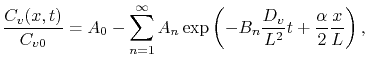
![$\displaystyle A_n = \frac{16n\pi\alpha^2[1-(-1)^n\exp(\alpha/2)]}{(\alpha^2+4n^...
...ymL}\right) + \frac{2n\pi}{\alpha}\cos\left(n\pi\frac{x}{\symL}\right) \right],$](img665.png)
![\includegraphics[width=\linewidth]{chapter_applications/Figures/SL_Cv_x=0_crop.eps}](img673.png)
![$\displaystyle S(0) = \left[ \left( \frac{\lambda_1\DV^1 - \lambda_2\DV^2}{\DV^2...
... - \DV^1\symElecField_1} \right) \frac{\kB\T}{\vert\Z\vert\ee} - 1\right]^{-1},$](img683.png)
![\begin{equation*}\begin{aligned}&\lambda_1 = -\frac{\vert\Z\vert\ee\symElecField...
...)^2 + \frac{1}{\DV^2\symVacRelTime_2}\right]^{1/2}. \end{aligned}\end{equation*}](img684.png)