Consider a simple ![]()
![]() m Cu long line, where the mechanical deformation, and consequently mechanical stress, accompanying electromigration is determined by the solution of (3.78)-(3.82).
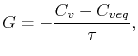
Here, the effect of vacancy annihilation/production on the strain rate is determined by
m Cu long line, where the mechanical deformation, and consequently mechanical stress, accompanying electromigration is determined by the solution of (3.78)-(3.82).
Here, the effect of vacancy annihilation/production on the strain rate is determined by
![\includegraphics[width=0.47\linewidth]{chapter_applications/Figures/K_stress_cathode.eps}](img692.png)
![\includegraphics[width=0.47\linewidth]{chapter_applications/Figures/K_stress_anode.eps}](img693.png)
|
At the anode end (![]() ) there is a depletion of vacancies, or an excess of Cu atoms, which leads to a compressive stress (negative). In turn, accumulation of vacancies at the cathode (
) there is a depletion of vacancies, or an excess of Cu atoms, which leads to a compressive stress (negative). In turn, accumulation of vacancies at the cathode (![]() ) driven by electromigration results in a tensile stress (positive).
The stress profile along the center of the line is shown in Figure 5.9.
The magnitude of the stress at the ends of the line gradually increases with time, developing the stress gradient which counters electromigration.
In steady state, the stress varies linearly along the line, and the electromigration flux is totally compensated by the back flux driven by the gradient of stress.
) driven by electromigration results in a tensile stress (positive).
The stress profile along the center of the line is shown in Figure 5.9.
The magnitude of the stress at the ends of the line gradually increases with time, developing the stress gradient which counters electromigration.
In steady state, the stress varies linearly along the line, and the electromigration flux is totally compensated by the back flux driven by the gradient of stress.
Figure 5.10 shows the development of the vacancy concentration at the cathode end with time.
This curve can be divided into three regions.
The first corresponds to the initial period of time, where a rapid increase in the vacancy concentration is observed. It is a quite short period and lasts about ![]() s only.
By this time the second period starts, where the vacancy concentration remains practically constant. This period lasts until about
s only.
By this time the second period starts, where the vacancy concentration remains practically constant. This period lasts until about
![]() s.
Kirchheim [53] called this period a quasi steady state period.
Finally, in the third period, the vacancy concentration increases at a low rate until the true steady state is reached. Typically, this is the longest period, lasting from hundreds until thousands of hours.
s.
Kirchheim [53] called this period a quasi steady state period.
Finally, in the third period, the vacancy concentration increases at a low rate until the true steady state is reached. Typically, this is the longest period, lasting from hundreds until thousands of hours.
The initial stress build-up closely follows the first period of increase of the vacancy concentration. As the quasi steady state is reached, the stress grows approximately linearly with time, shown in Figure 5.11. It corresponds to a period of transition from lower to higher values of stress. At first, the low stress does not affect the equilibrium vacancy concentration. However, as the stress magnitude increases, the equilibrium vacancy concentration also increases, which, in turn, affects the stress build-up due to the generation/recombination term given in (5.11). As a consequence, the third period is characterized by a non-linear increase of the stress until the true steady state is reached, as can be seen in Figure 5.12. The correspondence between these periods of vacancy development with mechanical stress build-up was already observed by Kirchheim [53].
![\includegraphics[width=0.85\linewidth]{chapter_applications/Figures/K_stress_linear.eps}](img698.png)
|
![\includegraphics[width=0.85\linewidth]{chapter_applications/Figures/K_stress_t.eps}](img699.png)
|
To sum up, high mechanical stresses can develop in a conductor line under electromigration. The stress build-up with time is a slow process, where high stresses develop after several hours, in contrast to the fast vacancy build-up observed in the results of Section 5.2.1. Moreover, the numerical simulation results reproduce the same characteristic behavior described by Kirchheim [53].
![\includegraphics[width=0.85\linewidth]{chapter_applications/Figures/K_stress_x.eps}](img694.png)
![\includegraphics[width=0.85\linewidth]{chapter_applications/Figures/K_Cv_t.eps}](img695.png)