The electron’s transport peculiarities determine the performance of most modern devices. In order to describe these peculiarities the band structure must be known. In other words the dependence of electron energy on wave vector k in different electron bands n, En(k) and relative positions of one band to another are decisive. Current level of technologies makes it possible to change the band structure of a material purposefully to achieve certain characteristics.
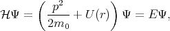
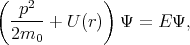
The energy spectrum of an electron in a crystal is determined by the Schroedinger equation
|
| (4.1) |
where U(r) is the periodic crystal potential and m0 is the electron rest mass.
To find the eigenfunctions and the eigenvalues of Equation 4.1 the two following task should be solved – determine the periodic potential and solve Equation 4.1 for the determined potential. Unfortunately the exact solution requires significant calculation recourses, thus approximate methods come into play. The task of finding the right kind of periodic potential for a given problem, is the most important part to obtain the correct solution. The second part of the solution is much more investigated. There are several methods available that allow to calculate the energy spectrum in metals and semiconductors with sufficient accuracy to reproduce experimental results.
The general idea behind most of the developed methods to solve Equation 4.1 is that every solution can be expanded in an infinite series by using a complete basis satisfying the same boundary conditions as the solution.
 | (4.2) |
The approximate solution can be obtained by taking a finite number of terms in the expansion. Functions Ψ1,
Ψ2, Ψ3, , Ψn are chosen to satisfy the boundary conditions. The following linear combination is taken for
approximation
, Ψn are chosen to satisfy the boundary conditions. The following linear combination is taken for
approximation
 | (4.3) |
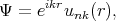
In order to understand how to choose proper functions Ψi(r) consider the following Bloch function
 | (4.4) |
This function has a plane wave factor. The plane wave is additionally modulated by factor unk(r). The factor unk(r) has the same period as the lattice. Close to atomic lattice sites the wave functions behave like the wave function for atoms, i.e. changes the Bloch amplitude fast. While far away from the atomic lattice sites the wavefunctions behave like plane waves and like atomic functions close to the sites.
The behavior of wave functions near the lattice sites and between the sites leads to the idea that either plane or spherical functions can be used in the linear combination (4.3). Based on this all methods that are used for band structure calculation are divided into two categories: variational methods and cellular methods.
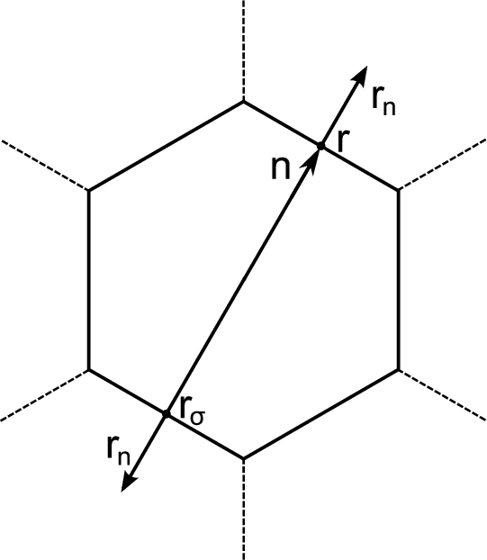
The cellular method was developed by Wigner and Seitz in 1933 [122]. The method utilizes the periodicity of the eigenfunctions of Equation 4.1, due to the periodic potential U(r). This periodicity makes it possible to restrict the task of finding eigenvalues and eigenfunctions to one primitive cell – the Wigner-Seitz cell. The Wigner-Seitz cell has a polyhedron shape that is limited by planes perpendicular to and passing through the midpoint of a line connected to an lattice point in the middle of the cell and its neighbors. Thus, the Wigner-Seitz cell built for an atom covers a region of space that is closer to the current atom than to the others. Such cells fill all the area (for two dimensional) or the volume (for 3D) of a crystal therefore it is enough to find a solution of Equation 4.1 in such a cell. The boundary conditions are the following
 | (4.5) |
 | (4.6) |
where r and rσ are location vectors of conjugate points on the surface of the Wigner-Seitz’s polyhedron, n is the translation
vector connecting these points or cell’s centers,  and
and  are normal derivatives at the point rσ and r, respectively, rn
is the outer normal for the surface of polyhedron.
are normal derivatives at the point rσ and r, respectively, rn
is the outer normal for the surface of polyhedron.
Equation 4.5 is the condition for periodicity. The Solution on the edge of the cell can be found by multiplying the solution at the opposite edge by the factor eikn. Equation 4.6 ensures solutions continuity and smoothness at the boundary of a cell.
The solution of the Schroedinger equation is sought in the form of a linear superposition of self-consistent atomic wave functions and radial functions. Such a representation of a wave function is valid under the assumption that the crystal potential in the small area around an atom inside each cell is symmetric. Wave function expansion coefficients are chosen in such a way that they meet the boundary conditions for the finite number of points at the surface of the cell. The described method has one considerable obstacle. Since the Wigner-Seitz cell usually has a complicated structure the use of boundary conditions in a direct way is almost impossible. Therefore, a simplified approach was developed. For this approach the boundary conditions are only being required to be satisfied in the middle of the edges. The results were not very precise, however, they were good qualitatively. Attempts to improve the results by including more points made the solution more complicated without significant improvement of the precision. To avoid the difficulties caused by the boundary conditions the simplest approximation can be applied. In this case a polyhedron is replaced by a sphere of the same volume
 | (4.7) |
where rs is the radius of Wigner-Seitz sphere.
The boundary conditions are then simplified to requirements for the wave function and its derivative continuity on the boundary of the sphere. Under these boundary conditions the solution is considerably simplified. However, such an approximation can not describe any state of a crystal. These conditions are only good enough for s-type states.
Variational methods reduce the solution of the differential equation (4.1) to the variational problem of the minimization of the functional Λ
 | (4.8) |
By substituting Equation 4.3 into Equation 4.1 and then multiplying by the complex conjugate wave function and integrating over the crystal volume one can get the following system of algebraic equations
 | (4.9) |
where  ji and Sji are written as
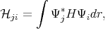 | (4.10) |
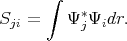 | (4.11) |
Here Sji≠δji since the functions Ψi and Ψj are not necessary orthonormal.
The system of equations (4.9) has a non-trivial solution only if determinant is equal to zero
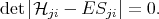 | (4.12) |
The characteristic equation (4.12) allows to find the eigenvalues, and then the eigenfunctions can be found by using Equation 4.9. Equation 4.12 has n solutions on E. The smallest solution is approximately equal to the energy of the lowest state. The higher solutions give energies of excited states. In general the quality of the solution at higher energies is worse than the lowest solution. The task of finding the eigenvectors and the eigenfunctions for Equation 4.1 by taking into account the boundary conditions Equation 4.5 and Equation 4.6 then can be reduced to a variational task of minimizing of functional
![∫
Λ[Ψ, Ψ*,E ] = Ψ *(H - E )Ψdr,](disser17x.png) | (4.13) |
where functions Ψ satisfy the boundary conditions.
A specific form of the characteristic equation (4.12) depends on the form of the functional (4.13), probe wave functions and boundary conditions. The order of the equation is determined by number of parameters ci, which is determined by number of basis functions Ψi that is used to get a good approximation of Ψ. Thus, the quality of the approximation depends on a good choice of probe functions Ψi.
The described approach is general and in order to solve the Schroedinger equation for a real crystal by a composition of wave functions consisting only of plane waves or only of atomic waves not quite satisfactory from a physical point of view.
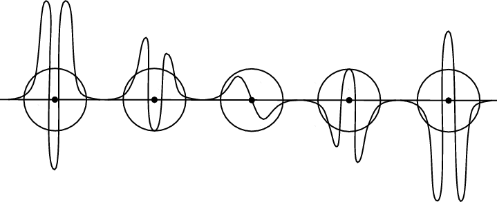
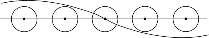
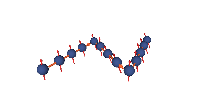
Actually, low lying bands are fully filled and described by wave functions that oscillate near the atom (Figure 4.2), while valence bands are characterized by wave functions equally distributed over the crystal (Figure 4.3). For the first case methods based on atomic waves are suitable to find a good solution for the equation. For the second case an approximation based on plane waves for the practically free electrons is suitable. The most interesting area for practical tasks is the intermediate region of the electron’s energy spectrum - for semiconductors it is the conduction and the valence bands.
A lot of efforts were taken to create a procedure for constructing basic wave functions that take into account both tendencies. An important point here is to build a procedure that allows to calculate wave functions in the most efficient (in the terms of numerical costs) way. The methods differ in the probe wave functions they are using.
All methods for the band structure calculation can be distinguished by the way the potential is built. Self-consistent methods use only atomic constants as parameters. Empirical methods use experimental data to get the best fit of the theoretical results in comparison to the experiments. Pure theoretical predictions of the band structure can be made only from self-consistent methods. The inconsistency of these predictions with regard to experimental results is a consequence of the approximations that are used for the calculations. The weakness of the empirical methods is their dependence on the parameters that are determined from experimental data.
Currently, all methods show approximately equal accuracy for energies below 0.5eV. Thus, the band structures obtained for energies below 0.5eV may be considered as correctly reproduced.
The method was first introduced by Seitz in 1935 [104], then it was extended by Luttinger [73], Kane [61] and Cardona [16]. As it was discussed earlier the eigenfunctions for one electron approximation for the Schroedinger equation
 | (4.14) |
are the Bloch functions
 | (4.15) |
where p = -iℏ∇ is the operator of the electron momentum, n is the band index, m0 is the electron rest mass, and the wave vector k is limited by the first Brillouin zone. By inserting Equation 4.15 to Equation 4.14 one gets
 | (4.16) |
The term  kp of Equation 4.16 is absent in Equation 4.14. This term can be considered as a perturbation. Thus, the term
is called kp-perturbation.
kp of Equation 4.16 is absent in Equation 4.14. This term can be considered as a perturbation. Thus, the term
is called kp-perturbation.
The solution of Equation 4.16 is sought as an expansion ukn in a complete set of functions. For a fixed k the set of ukn can be expanded as
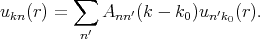 | (4.17) |
By isolating some part k0 from k, Equation 4.16 can be written in the following form
 | (4.18) |
where
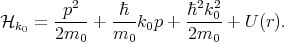 | (4.19) |
By substituting Equation 4.17 into Equation 4.18, multiplying by unk0*, and integrating over the elementary cell one can get the following system of equations
 | (4.20) |
where
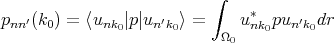 | (4.21) |
is the matrix element of momentum operator for the point k = k0. It is taken into account that functions u are orthogonal and normalized inside elementary cell
 | (4.22) |
The system of equations (4.20) is solvable if the following determinant is zero
![|[ ] |
|| -ℏ2- 2 2 -ℏ- ||
det | En(k0) - En (k) + 2m (k - k0) δnn′ + m (k - k0,pnn′(k0))| = 0.
0 0](disser30x.png) | (4.23) |
The secular equation (4.23) is used to find the eigenvalues En(k). To find out the dependencies of En(k), energies and matrix elements for all bands should be known for some k = k0. These values are usually obtained from experimental data.Pollak and Cordona [16] calculated En(k) by using the k⋅p method for a number of semiconductors (Si, Ge, GaAs, GaP, InP).
Frequently an exact solution of the Schroedinger equation can not be found. For a Hamiltonian that can be divided into two parts in such way that one part is much bigger than the other part a perturbation theory can be applied in order to find a solution. Consider the following Hamiltonian
 | (4.24) |
Here V is a small correction to the unperturbated Hamiltonian 0. The task that the perturbation theory
fulfills is to find approximate solutions for the eigenenergies E and the eigenfunctions Ψ of the following
equation
 | (4.25) |
provided that the eigenvectors E(0) and the eigenfunctions Ψ(0) for the unperturbated Hamiltonian are known, the eigenfunctions Ψn in the second order of approximation can be determined as
 | (4.26) |
where Ψn(1) and Ψ n(2) are the first and the second order correction of the eigenfunction written as [137]
 | (4.27) |
 | (4.28) |
with
 | (4.29) |
where V defined as an perturbation operator.
The eigenenergies En in the second order of approximation are written as
 | (4.30) |
with the first (En(1)) and the second (E n(1)) order corrections written as
 | (4.31) |
 | (4.32) |
The condition under which the perturbation theory is applicable is
 | (4.33) |
Namely matrix elements of the perturbation should be much smaller than the difference between the unperturbated energy levels.
However, even though the k⋅p method is valid for all values k, this method is most useful for the calculation of
the energy spectrum in the vicinity of the high symmetry point k0. If k - k0 is small enough then operator
 (k - k0,p) +
  in Equation 4.18 can be considered as a small perturbation to k0 and
 | (4.34) |
are a small correction to the energy En(k0).
By applying the perturbation theory to the equation for the energy close to the k0 point it can be written
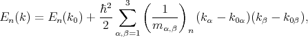 | (4.35) |
where  are the components of the inverse effective mass tensor.
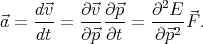
Consider a free electron that has rest mass m0 in a uniform electric field  . The force acting on the electron
is
. The force acting on the electron
is
 | (4.36) |
The force is directed against the field  and related to the electron acceleration by the following expression
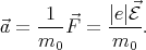 | (4.37) |
By taking into account the expressions for the velocity  and the impulse derivative over time
  for an electron in a
crystal in a uniform electric field
for an electron in a
crystal in a uniform electric field
 | (4.38) |
 | (4.39) |
acceleration can be rewritten as
 | (4.40) |
By generalizing Equation 4.40 for the three-dimensional case one gets
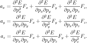 | (4.41) |
The set of values  =
=  , that connected acceleration and force are the second rank tensor
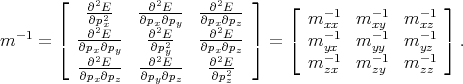 | (4.42) |
The tensor in Equation 4.42 is called inverse effective mass tensor.
Otto Stern and Walther Gerlach showed in 1922 that a beam of silver atoms directed through an inhomogeneous magnetic field would be forced into two beams [40]. This was consistent with the prediction of an intrinsic angular momentum and a magnetic moment by individual electrons. Classically this can be explained if the electron were a spinning ball of charge, and this property was called electron spin. This experiment confirmed the quantization of the electron spin into two orientations and made a major contribution to the development of the quantum theory of the atom.
The Schroedinger equation for a hydrogen atom is written as
 | (4.43) |
where =  + U is the Hamiltonian, p = -iℏ∇ is the momentum operator, U(r) = -|e|2∕r is the potential energy, m
0 is
the electron mass, |e| is the electron charge, Ψ(r) is the wave function (the square of the wave function determines
probability to find the electron in the volume dV ), E is the electron energy. The solution of Equation 4.43 leads to three
integer quantum numbers appear - n, l, ml. These numbers determine the eigenfunction for Equation 4.43 that describes
the probability for an electron position on atom. By taking into account the spin properties of the electron the fourth
quantum number ms appears. The spin magnetic quantum number ms characterizes the spin angular momentum of the
electron projection. In experiments it was shown that the electrons’ spin can have only two opposite projections on
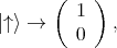
a fixed axis. For the electron, ms can have only two values +1∕2 and -1∕2. Usually this axis is chosen as
Z-axis. One of the spin orientations is parallel to the Z-axis and another is antiparallel to the chosen axis.
Thus, the two spin states are postulated as
+ U is the Hamiltonian, p = -iℏ∇ is the momentum operator, U(r) = -|e|2∕r is the potential energy, m
0 is
the electron mass, |e| is the electron charge, Ψ(r) is the wave function (the square of the wave function determines
probability to find the electron in the volume dV ), E is the electron energy. The solution of Equation 4.43 leads to three
integer quantum numbers appear - n, l, ml. These numbers determine the eigenfunction for Equation 4.43 that describes
the probability for an electron position on atom. By taking into account the spin properties of the electron the fourth
quantum number ms appears. The spin magnetic quantum number ms characterizes the spin angular momentum of the
electron projection. In experiments it was shown that the electrons’ spin can have only two opposite projections on
a fixed axis. For the electron, ms can have only two values +1∕2 and -1∕2. Usually this axis is chosen as
Z-axis. One of the spin orientations is parallel to the Z-axis and another is antiparallel to the chosen axis.
Thus, the two spin states are postulated as  and
and  . For the spin the following orthogonal eigenstates are
introduced
. For the spin the following orthogonal eigenstates are
introduced
 | (4.44) |
 | (4.45) |
The spin operator s = 
 is described by the following Pauli matrices
 | (4.46) |
 | (4.47) |
 | (4.48) |
An electron feels an atomic magnetic field while moving in a crystal. This field acts on the spin of the electron. The following Hamiltonian describes this impact
![HSO = --1---p[⃗σ × (∇V (x))].
4m2c2](disser70x.png) | (4.49) |
Here m is the free electron mass, c is the speed of the light in vacuum,  =
=  is the Pauli matrices,
V
is the Pauli matrices,
V  is the periodic potential, p is the momentum of the electron, and ∇V
  ∕|e| is the electron felt electric
field.
∕|e| is the electron felt electric
field.
Spin relaxation is the process characterizing the non-equilibrium spin vanishing. There are different mechanisms responsible for the spin relaxation: spin-orbital (Elliot-Yafet, D’yakonov-Perel’), electron-hole exchange interaction(Bir-Aronov-Pikus), and hyperfine interaction.
The Elliott-Yafet mechanism was proposed by Elliott [27] and Yafet [130]. The mechanism is important for small gap semiconductors with large spin-orbit splitting [10]. In electronic band structures the spin-up and the spin-down states are mixed by spin-orbit interaction [27]
 | (4.50) |
 | (4.51) |
The spin-up state contains spin-down and the spin-down state also contains a contribution from spin-up. However, the spin mixing is usually very small thus |bkn|≪|akn|. In the presence of such mixing spin relaxation events can be caused by any spin-independent scattering. In the absence of scattering events the spin state is conserved. This process is called the Elliott process. The Yafet process is due to a spin-orbit interaction in which the spin-orbit coupling of the conduction electrons to the lattice potential can be modulated by lattice vibrations. This leads to an interaction in which the spin of the electron is coupled to the quantum of the lattice vibrations (phonon).
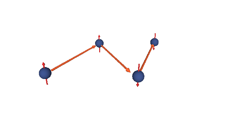
The D’yakonov-Perel’ relaxation mechanism [25] is an important spin-flip mechanism for conduction electrons. In semiconductor nanostructures without inversion symmetry there exists an effective spin-orbit contribution equivalent to a k-dependent effective magnetic field
 | (4.52) |
where  (k) is the spin precession frequency. The spin of moving electrons precess due to the effective magnetic field until
scattering occurs. After the scattering event the precession starts again but with a different
(k) is the spin precession frequency. The spin of moving electrons precess due to the effective magnetic field until
scattering occurs. After the scattering event the precession starts again but with a different  (k). At the scattering event the
momentum k changes randomly, hence spin precesses randomly after the scattering event. This relaxation has a notable
feature - stronger momentum scattering leads to a longer spin lifetime. The D’yakonov-Perel’ mechanism was found to be
dominated in Si quantum well structures but at low temperatures [31, 128].
(k). At the scattering event the
momentum k changes randomly, hence spin precesses randomly after the scattering event. This relaxation has a notable
feature - stronger momentum scattering leads to a longer spin lifetime. The D’yakonov-Perel’ mechanism was found to be
dominated in Si quantum well structures but at low temperatures [31, 128].
The Bir-Aronov-Pikus mechanism [8] describes the electron-hole exchange scattering that can lead to the electron spin relaxation in p-type semiconductors. Fluctuations in the effective hole concentration, due to different effective mass, produce a fluctuating effective magnetic field generated by the total spin of holes. This induces a precession of the electron spin around an instantaneous axis, analogously to the D’yakonov-Perel’ mechanism.
The forth mechanism responsible for the spin relaxation is hyperfine interaction. Hyperfine interaction is the magnetic interaction between the magnetic moments of electron and nuclei. This interaction is too small to cause effective spin relaxation of free electrons in bulk semiconductor [136, 90].