A Kolosov-Muskhelishvili Formulas

[next] [prev] [prev-tail] [tail] [up]

Appendix A
Kolosov-Muskhelishvili Formulas

The Kolosov-Muskhelishvili formulas provide the most convenient method to treat two-dimensional crack problems. This formulation allows us to consider stresses and displacements in therms of analytic functions of complex variables. Here, this formulation is derived for two-dimensional problems [70, 71].

A.1 Airy Stress Function

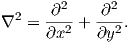
To derive the Kolosov-Muskhelishvili formulation it is necessary to introduce a new function, known as the Airy stress function. By using the stress-strain relations (2.46) together with the equilibrium equations (2.43) and the compatibility equations (2.45) described in Section 2.2 we can rewrite the compatibility condition as

2 ∇ (σxx + σyy) = 0,

(A.1)

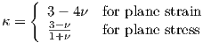
where the ∇² is the Laplace operator defined by

∂2 ∂2 ∇2 = ---2 +---2. ∂x ∂y

(A.2)

The Airy stress function ϕ is defined as

∂2-ϕ -∂2ϕ- ∂2-ϕ σxx = ∂y2, τxy = -∂x ∂y, σyy = ∂x2 .

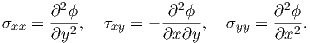(A.3)

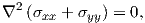
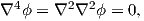
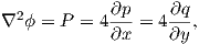
By using the relationships (A.3) in the equilibrium equations (2.43) it is possible to demonstrate that the equilibrium conditions are automatically satisfied by ϕ and (A.1) can be rewritten

∇4ϕ = ∇2 ∇2 ϕ = 0,

(A.4)

where ∇⁴ is the biharmonic operator and any function ϕ satisfying this equation is biharmonic.

A.2 Analytic Function and Complex Variable

Secondly, the Kolosov-Muskhelishvili method is formulated by describing two-dimensional elastic problems using analytic functions of complex variables. We define the position representation by the complex variable z, which in polar coordinates (r,θ) is given by

z = r(cosθ + isin θ) = reiθ, - iθ ¯z = r(cosθ - isin θ) = re ,

(A.5)

where z stands for the complex conjugation. (A.5) can also be described using the Cartesian coordinate system (x,y):

z = x + iy, z¯= x - iy.

(A.6)

A function of the complex variable z,

f(z) = f (x + iy) = f(x+ iy) = Ref(z) + iImf (z),

(A.7)

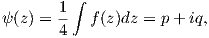
is said to be analytic at a point z₀, if it has a derivative at z₀ and at its neighborhood.

A.3 Complex Representation of the Airy Stress Function

To obtain the complex potential representation of the Airy stress function we introduce a function P

∇2 ϕ = P and ∇2P = ∇2∇2 ϕ = 0,

(A.8)

where

∂4 ∂4 ∂4 ∇2∇2 = ---4 + 2--2--2-+ --4-. ∂x ∂x ∂y ∂y

(A.9)

Due to the definition (A.4) P is harmonic. We define

P = Re {f(z)},

(A.10)

where f(z) is an analytic function defined by

f(z) = P + iQ.

(A.11)

The complex representation of the Airy stress function requires a further function

∫ ψ(z) = 1- f(z)dz = p + iq, 4

(A.12)

which is also analytic and its derivative corresponds to

′ 1 ψ (z) = 4-f(z).

(A.13)

By considering the Cauchy-Riemann equations we can describe ψ′(z) by

∂p ∂q ∂q ∂p ψ ′(z) = ---+ i---= ---- i--, ∂x ∂x ∂y ∂y

(A.14)

which allows us to obtain a relation between P and the functions p and q

∂p ∂q P = 4∂x- = 4∂y-.

(A.15)

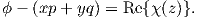
By using these relations we can rewrite (A.8) as

∇2 [ϕ- (xp + yq)] = 0,

(A.16)

where ϕ- (xp + yq) is harmonic and can be written as the real part of some analytic function. Therefore χ(z) can be chosen and is defined as

ϕ - (xp + yq) = Re {χ(z)}.

(A.17)

By employing the relation

xp + yq = Re {¯zψ(z)},

(A.18)

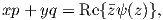
the complex potential representation of the Airy stress function is obtained

-- ϕ = Re {zψ(z)+ χ (z)}.

(A.19)

If we define

-- ---- ---- ---- Θ (z) = zψ (z )+ χ(z), and Θ(z) = zψ(z)+ χ (z),

(A.20)

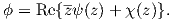
summing these equations, we obtain

-- -- -- ----- ---- Θ (z)+ Θ (z) = zψ (z)+ χ(z)+ zψ(z)+ χ (z) = 2Re {Θ(z)} = 2ϕ.

(A.21)

Equation (A.21) is employed in the next section to derive the Kolosov-Muskhelishvili formulas.

A.4 Stress and Displacement described by
Airy Stress Function

By using the definition of the Airy stress function (A.19), the stresses can be described by

∂2ϕ- -∂2ϕ- -∂-( ∂ϕ- ∂ϕ-) σxx + iτxy = ∂y2 - i∂x∂y = - i∂y ∂x + i∂y , 2 2 ( ) σyy - iτxy = ∂-ϕ-+ i-∂-ϕ = -∂- ∂ϕ-+ i∂ϕ- . ∂x2 ∂x∂y ∂x ∂x ∂y

(A.22)

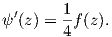
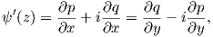
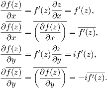For an analytic function f(z) the following relations are valid [70, 71]

∂f-(z-) ′ ∂z- ′ ∂x = f (z)∂x = f (z), ∂f-(z-) (-∂f(z))- ----- ------= ------ = f′(z), ∂x ∂x ∂f-(z-)= f ′(z)∂z-= if′(z), ∂y ∂y ∂f-(z-) (-∂f(z))- ----- ------= ------ = - if′(z). ∂y ∂y

(A.23)

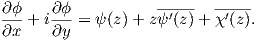
The differentiation of (A.21) with respect to x and y gives

∂ϕ -- ----- ----- ----- 2 ---= zψ ′(z)+ ψ (z)+ χ′(z)+ zψ ′(z)+ ψ (z)+ χ′(z), ∂x [ ----- ----- -----] 2 ∂ϕ-= i zψ ′(z)- ψ (z)+ χ′(z)- zψ ′(z)+ ψ (z)- χ′(z) , ∂y

(A.24)

where the second equation multiplied by i and summed to the first gives:

∂ϕ ∂ϕ ----- ----- ---+ i---= ψ (z)+ zψ ′(z)+ χ ′(z). ∂x ∂y

(A.25)

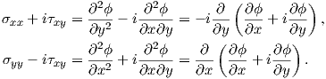
The equations from (A.22) can be rewritten using (A.25)

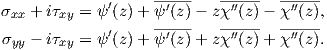′ --′-- -′′--- -′′-- σxx + iτxy = ψ (z)+ ψ-(z) - zχ-(z)- χ-(z), σyy - iτxy = ψ ′(z)+ ψ ′(z) + zχ′′(z)+ χ′′(z).

(A.26)

The sum of these two equations results in

[ ----] [ ] σxx + σyy = 2 ψ′(z) + ψ′(z) = 4Re ψ′(z )

(A.27)

and the subtraction of the first equation from the second produces

------ ----- σyy - σxx - 2iτxy = 2zψ′′(z)+ 2χ ′′(z).

(A.28)

Taking its complex conjugated results in

[-- ′′ ′′ ] σyy - σxx + 2iτxy = 2 zψ (x )+ χ (z) .

(A.29)

The two equations (A.27) and (A.29) are the complex potential representation of the stresses.

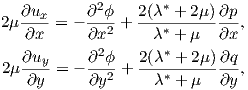
Further we derive the complex potential of the displacements. (2.44) and (A.3) can be substituted in (2.46) to give

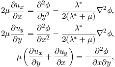∂ux ∂2ϕ λ* 2 2μ ∂x--= ∂y2-- 2(λ-* +-μ)∇ ϕ, 2 * 2μ ∂uy-= ∂-ϕ-- ---λ----∇2 ϕ, ∂y ∂x2 2(λ * + μ) (∂ux ∂uy) ∂2ϕ μ ----+ ---- = ------, ∂y ∂x ∂x ∂y

(A.30)

where

λ* = 3--κ-μ κ - 1

(A.31)

and κ is defined by

{ 3 - 4ν for plane strain κ = 3--ν for plane stress 1+ ν

(A.32)

and μ is the shear modulus.

By plugging

∇2 ϕ = P = 4 ∂p-= 4∂q-, ∂x ∂y

(A.33)

into (A.30) we obtain

∂u ∂2ϕ 2(λ* + 2μ) ∂p 2μ --x-= - --2-+ ---*------ --, ∂x ∂x λ + μ ∂x ∂uy- ∂2ϕ- 2(λ-* +-2μ)-∂q 2μ ∂y = - ∂y2 + λ * + μ ∂y,

(A.34)

which by integrating leads to

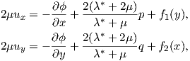∂ϕ- 2(λ-* +-2μ) 2μux = - ∂x + λ * + μ p + f1(y), * 2μuy = - ∂ϕ-+ 2(λ--+-2μ)q + f2(x), ∂y λ* + μ

(A.35)

where f₁(y) and f₂(x) represent rigid body displacements and can be neglected. This equation can be rewritten in complex form

( ∂ϕ ∂ϕ ) 2(λ* + 2μ ) 2μ(ux + iuy) = - ∂x-+ i∂y- + --λ* +-μ--ψ(z),

(A.36)

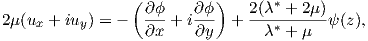
and recalling (A.25) we obtain

2μ(u + iu ) = κψ (z )- zψ′(z)- χ′(z), x y

(A.37)

which represent the complex potential of the displacements.

The Kolosov-Muskhelishvili formulas are given by the equations set (A.27), (A.29), and (A.37).

[next] [prev] [prev-tail] [front] [up]