In Chapter 3 the nanoindentation technique was applied in order to locate the areas with a
high concentration of mechanical stress in an open TSV. In these areas the probability of
device failure, such as cracking or delamination, is high. The bottom of the TSV under
consideration, which saw the highest stress build-up, consists of a multilayer structure which
represents the Al-based interconnection used in CMOS technology. In this section
we investigate how external forces, layer thicknesses, and the residual stress in the
layers can induce delamination at the interfaces which form the bottom of an open
TSV.
In order to understand the delamination failure it is first necessary to explain the theory
of cracks in bodies. The following theories are based on and described in detail in
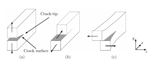
[37, 68, 69, 70, 71]. In continuum mechanics a crack is defined as a cut in a body which has its
end inside the body volume. This end of the crack is referred to as a crack-tip. Crack surfaces
are defined as the two opposite boundaries formed by the cutting plane and are generally
treated as traction-free. The crack-tip and crack surfaces are illustrated in Figure
4.1.
In a solid material a crack can propagate in three different modes:
- Mode I: Opening the crack opens normal to the crack plane due to a load
perpendicular to the crack surface.
- Mode II: Sliding the crack faces are displaced parallel to the crack surface and
perpendicular to the crack-tip due to a shear loading.
- Mode III: Tearing the crack faces are displaced parallel to the crack surface and
parallel to the crack-tip due to a shear loading acting in parallel to the crack tip.
These propagation modes can occur independently or in combination.
To fully understand the crack propagation modes it is necessary to analyze the crack-tip field
within a small region of radius R around the crack tip. Therefore the description of the crack-tip
field demands the specification of a hybrid Cartesian and polar coordinate system as shown
in Figure 4.2.
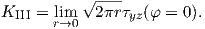
The mechanical analysis of the crack-tip field under mode I (cf. Figure. 4.1 (a)) will be
explained in the following and it is based on [37, 70, 71].
The derivation of the crack-tip field is achieved by employing the Airy stress function and
the Westergaard approach which are described in Appendix A and Appendix B,
respectively. The system analyzed is illustrated in Figure 4.2, where a set of in-plane Cartesian
coordinates x and y, and polar coordinates r or φ at the crack tip are chosen. A complex
representation z = x + iy of the coordinates is employed in the derivations.
A line crack with the following boundary conditions is considered:
- Very large stresses at the crack tip.
- Traction free crack surfaces.
The stresses σxx and σyy along the y = 0 plane can be expressed as
 | (4.1) |
where ZI(z) is the Westergaard function described in Appendix B and is employed to analyze
crack problems [70, 71]. The Westergaard function permits to analyze the stress field at the
crack tip by using a complex potential, as the Airy stress function, related to boundary
condition of the system. In the following derivations the argument of Z is omitted for better
readability and the subscript of Z indicates the crack mode. Because the strain energy in the
body has to be finite, the order of the singularity of stresses at the crack has to be of higher
order than z-1∕2. Therefore the solution of the crack problem can be written in the
form
 | (4.2) |
where g(z) is a function which does not diverge at the crack tip (z → 0). In this way the solution
permits to obtain σyy →∞ for z → 0, satisfying the first boundary condition. The second
boundary condition σyy = 0 for x < 0 and y = 0, is defined by
 | (4.3) |
which is satisfied if g(x) is real along y = 0.
The function g(z) close to the origin of the crack-tip can be represented by a Taylor
series
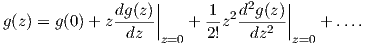 | (4.4) |
Close to the crack-tip the function g(z) is real and constant. This constant g(0) is related to the
stress intensity factor KI by
 | (4.5) |
which gives
 | (4.6) |
close to the crack tip. The subscript of the stress intensity factor KI indicates the crack mode.
K represents the magnitude of the crack tip stress.
The functions ZI and ZI′ necessary to describe the stresses near the tip can be expressed by
employing the polar coordinate representation of z = reiφ
![KI KI -iφ KI [ (φ ) ( φ) ]
ZI = √-----= √----e 2 = √----- cos -- - isin -- ,
2πz 2πr 2πr 2 2 [ ( ) ( )]
Z′ = -d-√KI---= - 1√KI--z- 32 = - √KI--1e- i3φ2-= - √KI---1--cos 3φ- - isin 3φ- .
I dz 2πz 2 2π 2 πr2r 2πr 2r 2 2](Main593x.png) | (4.7) |
Therefore the real and imaginary parts of the Westergaard function are
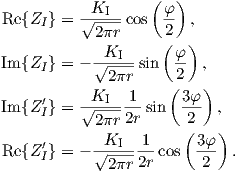 | (4.8) |
The stresses at the crack-tip can be described by using the Westergaard function (more detail in
Appendix B)
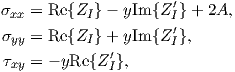 | (4.9) |
where A is an uniaxial stress that does not add singularity at the crack tip. If we do not consider
the higher-order terms, the stresses at the crack tip are given by plugging (4.8) into (4.9) (A is
set to 0)
![( ) [ ( ) ( )]
-KI--- φ- φ- 3φ-
σxx = √2-πr-cos 2 1- sin 2 sin 2 ,
K ( φ) [ ( φ ) ( 3φ )]
σyy = √--I--cos -- 1+ sin -- sin --- ,
2πr ( 2) ( ) 2 ( ) 2
τ = √KI---cos φ- sin φ- cos 3φ- ,
xy 2πr 2 2 2](Main598x.png) | (4.10) |
where y = r sin φ = 2r sin  cos
cos .
.
The displacements at the crack-tip are obtained by following the same procedure
(cf. Appendix B)
![KI √ ----[ (φ ) ( 3φ) ]
ux = 8μπ- 2πr (2κ- 1) cos 2- - cos 2-- ,
√ ---[ ( ) ( ) ]
uy = -KI- 2πr (2κ + 1)sin φ- - sin 3φ- ,
8μπ 2 2](Main603x.png) | (4.11) |
where for the plane strain, κ and σzz are defined by
 | (4.12) |
and for the plane stress, they are defined by
 | (4.13) |
where μ denotes the shear modulus.
With (4.10) and (4.11) stresses and displacements at the crack-tip for mode I
have been derived. These equations are valid for any cracked body under mode I,
where if the stress σyy is know, the stress intensity factor for mode I can be obtained
as
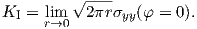 | (4.14) |
Since the approach is analogous for the other two modes only the end results are
given in the following. During mode II the stresses near the crack-tip are defined
by [37, 70, 71]
![( )[ ( ) ( ) ]
σxx = - √KII-sin φ- 2 + cos φ- cos 3φ- ,
2πr ( 2) ( ) 2( ) 2
-KII-- φ- φ- 3φ-
σyy = √2-πr-sin 2 cos 2 cos 2 ,
K ( φ) [ ( φ ) ( 3φ )]
τxy = √--II-cos -- 1- sin -- sin --- ,
2πr 2 2 2](Main609x.png) | (4.15) |
and the displacements by
![√----[ ( ) ( )]
ux = KII- 2πr (2κ+ 3)sin φ- + sin 3φ- ,
8μπ [ 2( ) 2( )]
-KII√ ---- φ- 3φ-
uy = -8μ π 2πr (2κ - 3)cos 2 + cos 2 .](Main612x.png) | (4.16) |
If the stress τxy is known the stress intensity factor for mode II can be obtained as:
 | (4.17) |
For mode III the stresses near the crack-tip are
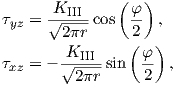 | (4.18) |
and the corresponding displacement is
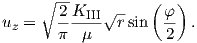 | (4.19) |
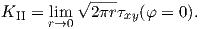
Also here a stress intensity factor can be derived if the stress τyz is known
 | (4.20) |
In this section the fundamental equations required to describe cracks in the interface between
two materials with different material properties, also referred to as delamination, are given. The
reported theory is based on [37, 70].
The concept of the intensity factor K, described in the previously section, cannot be easily
applied, because the crack-tip in the case of delamination field has a different form compared to
a crack in a single homogeneous material.
Delamination is illustrated in Figure 4.3. A bimaterial crack lies at the interface between
two materials with elastic constants E1, ν1 and E2, ν2. This particular problem is
analyzed by using an eigenfunction expansion method [37, 70]. For the description of the
crack-tip field, a plane strain condition is considered, the complex variable method is
employed (cf. Appendix A), and polar coordinates at the crack-tip are defined.
The first boundary condition of the problem is that the crack surfaces (φ = ±π) are
traction-free
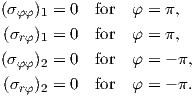 | (4.21) |
The second boundary condition is the continuity of the stress field and the displacement field at
the interface (φ = 0)
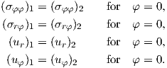 | (4.22) |
These boundary conditions represent a system of equations where a general solution has to be
obtained. One possible approach is to describe the problem through the Airy stress
function ϕ for Material 1 and for Material 2. The Airy stress function satisfies the
equilibrium equations (2.43) and therefore the compatibility equation (2.45) is given
as
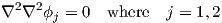 | (4.23) |
with the Nabla operator ∇2 defined as
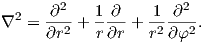 | (4.24) |
To obtain the solution of the boundary conditions the variables of the stress function have to be
separated in the following way
 | (4.25) |
where λ is the eigenvalue to be determined and Fj(φ) are the eigenfunctions of the biharmonic
operator in (4.23) [70].
If we insert (4.25) into (4.23), we obtain
 | (4.26) |
where the solution of the differential equations (4.23) can be obtained by using an Ansatz
leading to [72]
 | (4.27) |
where aj,bj,cj,dj are unknown constants.
By using (4.25) and the Airy stress in polar coordinates [70], the stress components are
described by
![2 [ ]
(σrr)j = 1-∂-ϕj-+ 1-∂ϕj-= rλ-1 F ′j′ (φ) + (λ + 1)Fj(φ) ,
r2∂ φ2 r ∂r
∂2ϕj λ-1
(σφφ)j = ∂r2--= r λ(λ + 1)Fj(φ),
1 ∂2ϕ 1 ∂ϕ
(σrφ)j = -------j+ -2---j= - λrλ-1F ′j(φ ),
r ∂r∂φ r ∂ φ](Main636x.png) | (4.28) |
and the displacements in polar coordinates [70] by
![1
(ur)j = ----rλ{- (λ + 1)Fj(φ)+ (1 + κj)[cj sin(λ - 1)φ + dj cos(λ - 1)φ]},
2μj
(u ) = -1--rλ{- F ′(φ )- (1+ κ )[c cos(λ- 1)φ - d sin(λ - 1)φ ]}.
φj 2μj j j j j](Main639x.png) | (4.29) |
Equations (4.28) and (4.29) are further plugged into the boundary conditions (4.21) and
(4.22)
![a1 sin(λ + 1)π + b1 cos(λ + 1)π + c1 sin(λ - 1)π + d1cos(λ - 1)π = 0,
- a2sin(λ+ 1)π + b2cos(λ + 1)π - c2 sin(λ - 1)π + d2 cos(λ - 1)π = 0,
a1(λ + 1)cos(λ+ 1)π - b1(λ+ 1) sin(λ + 1)π
+c1 (λ - 1)cos(λ - 1)π - d1(λ - 1)sin(λ- 1)π = 0,
a2(λ + 1)cos(λ+ 1)π + b2(λ+ 1) sin(λ + 1)π
+c (λ - 1)cos(λ - 1)π + d (λ - 1)sin(λ- 1)π = 0,
2 2
b1 + d1 = b2 + d2,
a1(λ + 1)+ c1(λ - 1) =( a2(λ +) 1)+ c2(λ - 1),
(1+ κ1)c1 = μμ12(1+ κ2 )c2 + μμ12 - 1 [(λ+ 1)a2 + (λ- 1)c2],
(1+ κ )d = μ1(1 + κ )d - (μ1 - 1) (λ + 1)[b + d ].
1 1 μ2 2 2 μ2 2 2](Main640x.png) | (4.30) |
A non-trivial solution of the system of equations (4.30) for the unknown coefficients aj,bj,cj,
and dj exists if the determinant of the system 8×8 vanishes. The solution of the system of
equations leads to
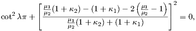 | (4.31) |
where this equation only has complex solutions for λ (real solution results only if a homogeneous
material is considered Material 1 = Material 2). Therefore a physically solution [70] is obtained
for the set of eigenvalues:
 | (4.32) |
where
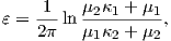 | (4.33) |
with μi = Ei∕2(1 + νi), κi = 3 - 4νi and ε the bimaterial constant.
The field which dominates as r → 0 (forming a singularity of the stress at the crack-tip)
corresponds to the eigenvalue with the smallest real part
 | (4.34) |
Taking into account
 | (4.35) |
and using (4.28) and (4.29), and considering (4.34) the stresses and displacements can be
approximated to
![σrr,σ θθ,σrθ ~ r-1∕2[cos(εlnr) + isin(εln r)], ur,uθ ~ r1∕2[cos(εlnr)+ isin(εlnr)].](Main650x.png) | (4.36) |
It is clear that the typical 1∕ -type singular behavior for the stresses and the displacements is
present at the bimaterial crack-tip. Unlike for a homogeneous body, these quantities oscillate,
with increasing amplitude, while approaching the crack-tip.
-type singular behavior for the stresses and the displacements is
present at the bimaterial crack-tip. Unlike for a homogeneous body, these quantities oscillate,
with increasing amplitude, while approaching the crack-tip.
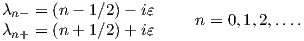
The crack tip stresses (in Cartesian coordinates) can be expressed by introducing the stress
intensity factors [37, 73] as:
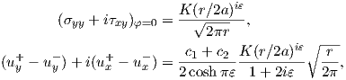 | (4.37) |
where 2a indicates an arbitrary reference crack length, the sign + and - are the upper and
lower surface of the crack tip, respectively (Figure 4.3), and K is the stress intensity factor
which can be separated in a real and an imaginary part:
 | (4.38) |
and
 | (4.39) |
The stress intensity factors and the length 2a are weighted by the material constant ε and
therefore a decomposition into purely mode I and mode II is not possible. This can be seen if
using relation (4.35) we write the stresses at the interface from (4.37) in the following
form
![1
σyy = √-----{K1 cos[ε ln(r∕2a)]- K2 sin[ε ln(r∕2a)]},
2πr
τxy = √-1---{K1 cos[ε ln(r∕2a)]+ K2 sin[ε ln(r∕2a)]}.
2πr](Main659x.png) | (4.40) |
The stress intensity factor K1 is associated with the normal and the shear stresses in the
interface, which is also true for K2 since during delamination both modes are inseparably
connected to each other. In the homogeneous material case K1 and K2 correspond to
K
IandK_II,respectively.
The energy release rate G is a fundamental concept in fracture mechanics [37, 70, 71]. This
quantity is the released energy dΠ during an infinitesimally small crack advance dA (A indicates
a crack area in 3D and a crack length in 2D)
 | (4.41) |
The total potential energy Π is composed of the strain energy U and the potential of external
forces V
 | (4.42) |
where U is defined by
 | (4.43) |
where A0 is the initial area of the crack. V is defined by
 | (4.44) |
W in (4.43) is the strain energy density given by
 | (4.45) |
where σij denotes the components of the stress tensor and εij the components of the strain
tensor [74]. In (4.44) Ti indicates a prescribed traction on Γt and ui the corresponding
displacements (cf. Figure 4.4). If the body is not subjected to external tractions the potential
energy is equal to the strain energy Π = U.
In two-dimensional problems, dΠ is related to the crack extension and therefore by
considering an infinitesimally small crack extension da, G is defined by
 | (4.46) |
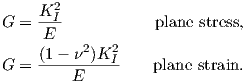
For a homogeneous material and assuming the linear elastic case G can be expressed in
terms of stress intensity factors, where G can describe a single mode or a combination of
modes.
We derive G for mode I (cf. Figure 4.1 (a)), where the stress before the crack elongates is
given by σyy and the displacement after the crack has elongated is given by uy along y = 0. The
strain energy generated over an increment of crack extension of length Δa is given
by
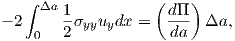 | (4.47) |
where the minus sign indicates that the stresses and displacements act in opposite directions
during relaxation and the factor of 2 refers to the two crack surfaces. By using the definition of
G (cf. (4.46)) and by considering a crack extension of a small length Δa in the limit Δa → 0, the
energy release rate for mode I is calculated
 | (4.48) |
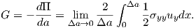
In the current problem, (4.6) is employed to describe the stress and displacement of
interest
 | (4.49) |
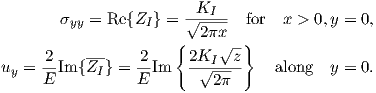
It is necessary to consider the displacement of interest which corresponds to the new crack
length. Therefore x = Δa and z = -(x- Δa) + iy,y = 0; therefore, the displacement of interest
is
 | (4.50) |
By plugging the stress (4.49) and the displacement (4.50) into (4.48) G can be obtained
 | (4.51) |
For modes II and III the same derivation can be carried out, leading to
 | (4.52) |
for mode II and to
 | (4.53) |
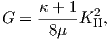
for mode III. If a general crack loading is taken in consideration, all three modes are present and
G is described by
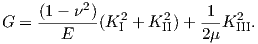 | (4.54) |
For delamination, G can derived by applying the same approach resulting in
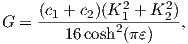 | (4.55) |
where c1 and c2 are described by (4.39), and ε by (4.33). Here G is uniquely determined by both
stress intensity factors K1 and K2.
During the fracture process new surfaces are generated [37, 71]. During the crack process the
material is separated along the fracture surface dA, which can be divided into the upper dA+
and lower dA- surface of the crack. During the creation of a crack expansion of dA, the energy
required to generate the fracture is given by dΓ. During the material separation due to cracking
dΓ is given by
 | (4.56) |
where γ is the fracture surface energy usually considered to be constant and the factor of 2
stands for the two surfaces of the crack.
If we consider a quasi static fracture process of an elastic body the balance of the energy in
play reads
 | (4.57) |
thus during the fracture process the change of the potential Π due to an external or
internal force and the fracture energy Γ sum up to zero. Using (4.56) and (4.41) we can
write
 | (4.58) |
with Gc = 2γ. Expression (4.58) can be understood as a condition for crack propagation. If
the released energy is equal to the energy needed for the fracture process the crack
will advance. This fracture criterion is know as Griffith’s fracture criterion [69] and
it is applicable for homogeneous materials. For the relation between G and Ki (i
indicates the crack mode) this criterion can be used for any combination of crack
modes.
The fracture criterion can also be described for bimaterial cracks. In Section 4.1.2 it was
shown that during delamination mode I and mode II always act together. G depends on K1 and
K2 and therefore the fracture criterion is based on both modes. The phase angle
Ψ of the mixed mode characterizes G; therefore, the fracture criterion is described
as
 | (4.59) |
The term Gc(i)(Ψ) is the fracture toughness and is a function of the phase angle Ψ. The fracture
resistance of the interface has to be experimentally measured.
The evaluation of the energy release rate G can be used to predict the crack or delamination
propagation. In this section the various procedures to calculate G are described. These
methodologies are then applied to the TSV structure in Section 4.4 and Section
4.5.
In linear fracture mechanics the value G can be obtained by applying the J-Integral
method [74, 75, 76].
The value of the J-Integral is equal to the energy which is dissipated by the fracture. The
J-Integral method is applicable for systems obeying linear-elastic fracture mechanics as well as
for materials with an inelastic behavior. The J-Integral is evaluated along a path Γ around the
crack-tip of the cracked body. The path can be arbitrary chosen as long as the crack-tip is inside
the region surrounded by the path [76].
The definition of the J-Integral is given by
 | (4.60) |
where W is the strain energy density, Ti are the components of the traction vector, ui are the
components of the displacement vector, and ni are the components of the unit vector
perpendicular to the integration path (Figure 4.5). The strain energy density is the work per
unit volume done during the elastic deformation of a material and is defined by (4.45).
For linear elastic materials, introducing (2.37) into (4.45), W is defined by
 | (4.61) |
The traction vector is defined by
 | (4.62) |
Considering a straight bond line, the standard J-Integral, primarily developed for problems
of single homogeneous materials, can also be applied to bi-material interfaces [37, 76].
The energy release rate G can be calculated by determining the values K1 and K2 from (4.55).
These values are obtained by regression analysis fitting. Regression analysis permits to obtain
unknown parameters by employing fitting functions. One of the most common approaches is the
least squares method, where through the minimization of the sum of squared residuals (residual
is the difference between an observed value and the fitted value provided by a model) the fitting
parameters can be obtained [77].
The stress intensity factors are obtainable by using the stress at the head of the right side of
the crack-tip (cf. Figure 4.3) which is described by (4.40). The equation for σyy is
multiplied by cos[εln(r∕2a)] and added to the equation for τxy previously multiplied by
sin[εln(r∕2a)] [78]. The resulting equation is denoted as σ1 and represents the combined
stress
![-K1---
σ1 = σyy cos[εln(r∕2a)]+ τxysin[εln(r∕2a)] = √2πr-.](Main712x.png) | (4.63) |
An additional combined stress σ2 can be obtained by multiplying τxy with cos[εln(r∕2a)]. An
addition to the product of σyy and sin[εln(r∕2a)] leads to
![σ2 = - σyy cos[εln(r∕2a)]+ τxysin[εln(r∕2a)] = √-K2-.
2πr](Main713x.png) | (4.64) |
The values σ1 and σ2 can be calculated using σyy and τxy, which can be obtained from FEM
simulations. The stress intensity factors K1 and K2 are calculated by a regression of σ1 versus r
and σ2 versus r [68, 78]. The values K1 and K2 can be further used to calculate G
using (4.55).
In this section the J-Integral method was employed to predict delamination failure at the TSV
bottom. The study was carried out by means of simulation, which is based on the evaluation of
the J-Integral at different interfaces. These simulations enable the determination of the
structures with the lowest failure probability.
The study of delamination in TSVs is necessary, because the delamination can increase the
probability of cracking or corrosion of the conducting layer (W) or lead to rupture of
sidewall oxide isolation. To limit these problems different factors were analyzed to
understand how they can influence delamination, and the mechanical stability of the
device.
The existence of mechanical stress can be sufficient to degrade the performance and
to induce crack or delamination in the TSVs [79]. In Section 3 the critical areas
where a mechanical failure of the TSV can be assumed were found. One of these
areas is the bottom of the TSV sidewall which consists of various interfaces between
different material films with different thicknesses and mechanical properties. At these
interfaces the possibility of delamination leading to failure of the device needs to be
considered.
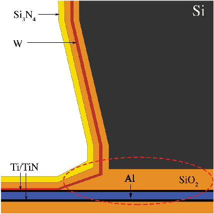
Figure 4.6 depicts the open TSV studied [29, 80, 81]. Different factors such as the
residual stress of the films, the film thicknesses, and the external forces influence the
failure of the device. By analyzing these factors the critical mechanical and geometrical
conditions which influence G, and thereby the probability of delamination, can be
studied.
The energy release rate G was calculated for the different interfaces at the bottom of the TSV
by using COMSOL Multiphysics [62]. Considering the bottom of an open TSV as free to bend,
cracking or delamination of the layers has to be expected under the sidewall (cf. red circled
region Figure 4.6).
Two-dimensional simulations for the structure shown in Figure 4.7 were carried out. All
the layers have a length w of 20 μm and the thicknesses of the layers were varied according to
the values given in Table 4.1.
All the materials were assumed to be linear elastic and isotropic. The failure of the
interconnection in the area under the sidewall was studied; therefore, the top layer of the
simulation space was assumed mechanically fixed as the sidewall of the TSV was fixed.
Furthermore, a downward force was applied on the bottom of the system and the bottom of the
TSV was considered free to bend (cf. Figure 4.7). The simulations were started with
a small initial crack length a and gradually increased until a predefined value was
reached.
The four interface systems found in the open TSV are Ti/Al, SiO2/TiN, SiO2/W, and
Si/SiO2. For the prediction of failure due to delamination, the values G are compared to critical
values Gc taken from [82, 83, 84, 85] and showed in the Table 4.2.
Calculations were carried out for different ratios of crack length a and layer width w. All
simulations start with a crack of length 0.5 μm which was gradually increased by steps of 0.5 μm
until 3 μm was reached.
|
|
|
|
|
|
| Layer | Ti/TiN | SiO2 | Al | W | Si |
|
|
|
|
|
|
| Thickness (μm) | 0.05-0.2 | 0.3-1.4 | 0.3-0.6 | 0.04-0.16 | 5 |
|
|
|
|
|
|
| |
Table 4.1: Thickness of layers employed.
|
|
|
|
| Interface | SiO2/TiN | Si/SiO2 | SiO2/W |
|
|
|
|
| Gc (J/m2) | 1.9 | 1.8 | 0.2-0.5 |
|
|
|
|
| |
Table 4.2: Critical values Gc for the considered interface.
By varying the following factors their influence on G was investigated:
- Residual stress: The stress was simulated by adding an initial stress in each
considered layer. It was introduced by setting σxx and σyy to the assumed stress
values. The residual stress in the layer is due to the combination of the film deposition
process and thermal processes. Small changes in residual stress influence the value
of G.
- Thicknesses of the layers: The thickness of the layers influence G and different
values were employed to find the critical condition for the delamination.
- External force: It can represent extra mechanical stress during the fabrication
processes (for example, during bonding between dies or between the interposer layer
and die [14]), or an accidental load, for example due to the presence of dust particles.
G was calculated by employing the J-Integral method (Section 4.3.1) where the integral path Γ is
displayed in Figure 4.7. Because the experimental critical values of Gc found in literature have
a larger range of phase angles Ψ and because the main mode which acts in the considered
structure is unknown, only G was evaluated in this study, without investigate the value of Ψ.
Therefore, the failure prediction is made by comparing G from the simulations with
Gc.
In all the plots shown (Figures 4.8-4.23), the x-axis represents the ratio a∕w, the y-axis the
considered factors, and the z-axis the calculated G. For the residual stress and thickness
analyses a downward force of 110 mN was applied (F in Figure 4.7).
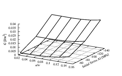
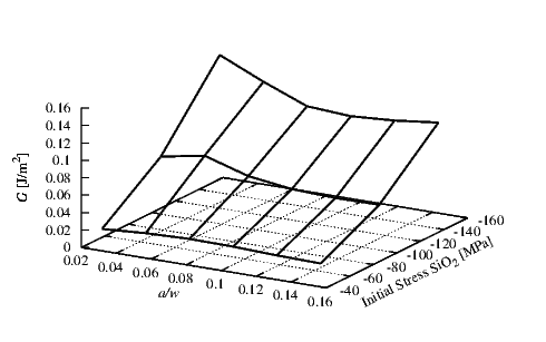
In Figure 4.8 the G values for the interface between Ti and Al are plotted.
The initial stress in the Al was assumed to be compressive. Inside the Ti a constant
compressive initial stress σTi of 50 MPa was used. For the Ti a thickness hTi of 0.15
μm and for the Al a thickness hAl of 0.5 μm were set. The effect of the ratio a∕w
on G is small compared to the influence of the initial stress. This shows that the
probability of a failure is effectively reduced by a decrease in the initial stress in the Al
layer.
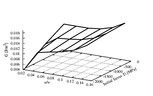
Figure 4.9 depicts the G value for an interface between Ti and Al where the initial stress in
the Ti was varied. For the Ti a thickness hTi of 0.15 μm and for the Al a thickness hAl of 0.5
μm were set. A compressive stress σAl of 100 MPa was set in the Al layer. A reduction in the
initial stress in Ti leads to an increase in the energy release rate; therefore, in contrast to
Figure 4.8 the decrease in the initial stress in the Ti layer can lead to a delamination
propagation. The increase of the crack length does not significantly influence G. For this
interface no value of Gc to compare with our values were available in literature. Nevertheless the
G values are very small thus we can assume no delamination failure for this interface.
Figure 4.10 shows the behavior of G at the interface between Si and SiO2. Thicknesses of 5
μm and 1.4 μm for Si (hSi) and SiO2 (hSiO
2) were used, respectively. The critical value Gc was
found to be 1.8 J/m2 [83]. All the points are far below the critical value. A slight
decrease of G with an increase of the crack length is observable. This shows the stability
of this interface for every crack length and for every initial stress in the SiO2 layer.
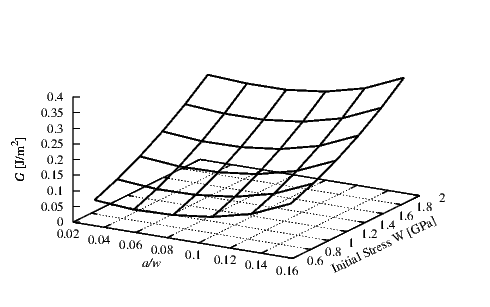
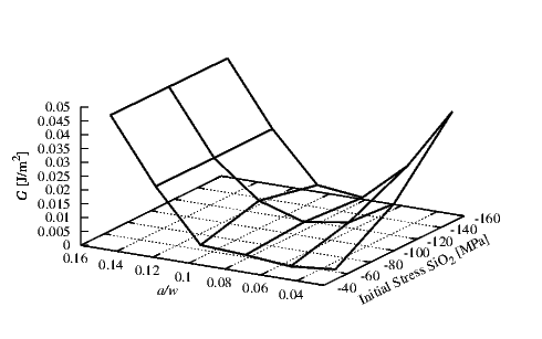
The behavior of G at the SiO2/W interface is shown in Figure 4.11 for thicknesses of 0.4
μm and 0.1 μm for the SiO2 (hSiO
2) and the W (hW) layers, respectively. In the SiO2
an initial compressive stress σSiO
2 of 100 MPa was assumed. The simulations were
carried out for different tensile initial stresses in the W layer. The Gc according to [84]
is in the range of 0.2-0.5 J/m2 and therefore quite small compared to G obtained
for the SiO2/W interface. For this system the influence of the a∕w ratio variation
is small compared to the initial stress variation. There is a constant increase in G
with an increase in the initial tensile stress in the W layer. Initial stresses above 1.25
GPa will lead to delamination at all a∕w ratios and therefore to the failure of the
device.
In Figure 4.12 the interface SiO2/W was also taken in consideration. An initial
tensile stress σW of 1.25 GPa and a thickness hW of 0.1 μm were used for the W
layer. Different initial compressive stresses in the SiO2 using a thickness hSiO
2 of 0.4
μm were simulated. An increase in G is observable for increasing crack lengths a.
In contrast to the behavior of G due to a varying initial stress in the W layer, here
the variation of G with respect to the variation of the initial stress in the SiO2 is
negligible. Only at high crack lengths is the modeled G value close to the critical Gc.
Therefore, the main influence to the stability of this interface is connected to the crack
length.
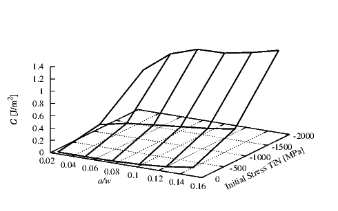
Figure 4.13 shows the behavior of G at the interface SiO2/TiN. Here thicknesses of 1 μm
and 0.15 μm for the SiO2 (hSiO
2) and TiN (hTiN) were used, respectively. A compressive stress
σSiO
2 of 100 MPa was used for the SiO2 layer. Critical value Gc for this interface was found to
be 1.9 J/m2 [82]. In this configuration the a∕w ratio does not cause failure at the
interface. The main effect which can be the cause of problems in this interface is the
initial stress in the TiN. A constant increase of G related to the initial stress can be
observed.
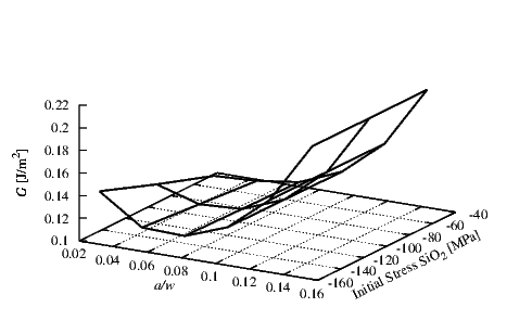
In Figure 4.14 the SiO2/TiN interface was analyzed. The thickness of 1 μm for the SiO2
(hSiO
2) layer and 0.15 μm for the TiN (hTiN) layer with a compressive initial stress
σTiN of 50 MPa for the TiN were chosen. By varying the a∕w ratio in the range
0.08 to 0.1 a minimum G at high initial stresses is found. This behavior results in a
high G for short and long crack lengths. This means that the presence of a crack
in the interface does not support the propagation, provided that the length of the
initial crack does not exceed a certain critical value. Under the modeled variation
configuration and load delamination will not occur as the values of G are below the critical
value.
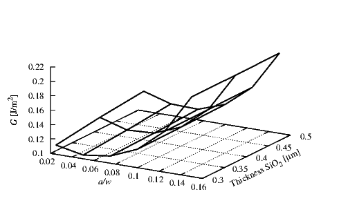
In Figures 4.15-4.19 the calculated G for different layers thicknesses is shown. In this section
the influence of the layer thicknesses are investigated. The results for the SiO2/W interface are
presented in Figure 4.15. For the SiO2 layer a thickness hSiO
2 of 0.4 μm and a compressive
stress σSiO
2 of 100 MPa were used. In the W layer a tensile stress σW of 1.25 GPa was applied.
The effect of the W thickness is highly relevant because a high increase of G is observed at long
crack lengths and small thicknesses. For large thicknesses of W the calculated G is in the
range of the Gc and for this condition we can expect delamination to take place.
Figure 4.16 shows the behavior of G at the SiO2/W interface. Here a thickness hW of 0.1
μm for the W was set. A compressive stress of 100 MPa in the SiO2 (σSiO
2) layer and a tensile
stress of 1.25 GPa in the W (σW) layer were used. The thickness of the SiO2 does not appear to
have a significant influence on G and the increase in G is only attributed to the a∕w
ratio.
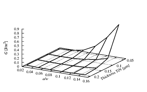
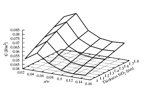
In Figure 4.17 the results at the interface between SiO2 and TiN for different TiN
thicknesses are displayed. A layer thickness hSiO
2 of 1 μm and a compressive initial stress of 100
MPa for the SiO2 (σSiO
2) and a compressive initial stress of 50 MPa in the TiN (σTiN)
were chosen. For this interface at very small thicknesses and at long crack lengths
there is an important increase in G which can exceed the critical Gc of 1.9 J/m2
[84].
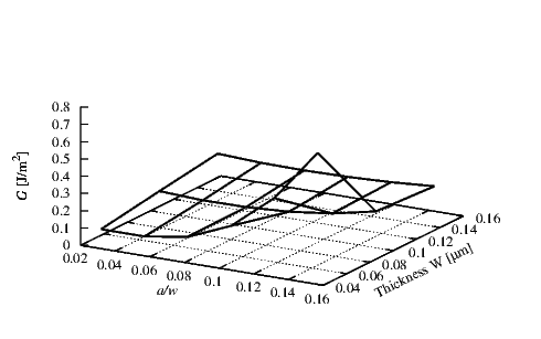
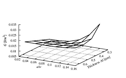
In Figure 4.18 the interface between the Ti and Al for different thicknesses were studied. A
thickness hTi of 0.15 μm and a compressive initial stress σTi of 50 MPa for the Ti
was used. A compressive stress σAl of 100 MPa for the Al was chosen. The critical
energy release rate for this interface is not available in literature. We can assume
that the delamination will not appear because the calculated values of G are very
small. A significant increase in G is noted only at small thicknesses of the Al and at
high crack lengths. For the other configurations the G remains almost unchanged.
In Figure 4.19 the G values of the interface between Si and SiO2 are reported. An initial
compressive stress σSiO
2 of 100 MPa in the SiO2 was used. For the Si layer a thickness hSi of
5 μm was set. The thickness variation of the SiO2 does not produce high value of G.
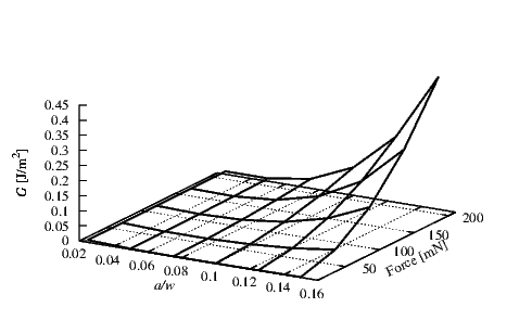
The effects of different forces on the system are presented in Figures 4.20-4.23. In these
simulations different forces in the range of 10-210 mN were applied.
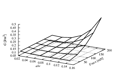
The behavior of G at the SiO2/W interface is shown in Figure 4.20. A thickness of 0.4 μm
for the SiO2 (hSiO
2) layer and a thickness of 0.1 μm for the W (hW) layer were employed. In
the SiO2 a compressive initial stress σSiO
2 of 100 MPa and in the W a tensile stress σW of
1.25 GPa were applied. The simulations were carried out for different forces. The Gc is in the
range of 0.2-0.5 J/m2 [84] and therefore small in comparison to the values of G obtained for the
SiO2/W interface. For this system delamination is expected only when a force over 100 mN is
applied.
In Figure 4.21 the G values of the interface between Si and SiO2 are plotted against the
a∕w ratio. An initial compressive stress σSiO
2 of 100 MPa in the SiO2 with a thickness hSiO
2 of
1.4 μm were used. For Si a layer thickness hSi of 5 μm was set. The effect of a force variation is
small compared to the influence of the a∕w ratio. In this interface for smaller crack
lengths the values of G are larger than for long crack lengths. The critical Gc value
of 1.8 J/m2 [83] for this interface is much larger than those calculated in the given
simulations.
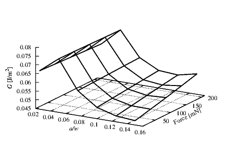
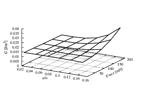
The G values of the interface between the SiO2/TiN are shown in Figure 4.22. Thicknesses
of 1 μm and 0.15 μm for the SiO2 (hSiO
2) and TiN (hTi) were used, respectively. A compressive
stress of 100 MPa for the SiO2 (σSiO
2) and 100 MPa for the TiN (σTiN) were applied. Here G
increases with the increase in the crack length and the applied force. The calculated values of G
are much lower than Gc, therefore we can expect delamination only for large applied
forces.
In Figure 4.23 the G values obtained for the interface between the Ti/Al are reported. For
the Ti layer a thickness hTi of 0.1 μm and initial compressive stress σTi of 50 MPa were
employed. The Al layer was assumed to have a thickness hAl of 0.5 μm and an initial
compressive stress σAl of 100 MPa. The G values obtained are very small therefore no
delamination can be supposed for this interface.
The impact of the layer thicknesses, the residual stresses, and the applied forces on the energy
release rate G were investigated and are summarized in Table 4.3.
In Section 4.4.3.1 the effects of the films’ residual stresses on G were investigated. In the
SiO2/W interface, a high probability of delamination propagation occurs when, due to
the deposition process and thermal processes, the W layer exhibits high values of
residual stress. In addition, the presence of defects, generated during film deposition
and resulting in the presence of cracks at the interface, increase the probability of
delamination failure. The SiO2/TiN interface shows the possibility of delamination
propagation only for high values of compressive initial stress in the TiN layer. The
variation of initial stress in the SiO2 does not produce high G values decisive for
mechanical failure. The Si/SiO2 interface remains stable for every crack length and residual
stress. Although the critical energy release rates are not available in literature for
the Ti/Al interface, a qualitative estimation of the delamination can be given. As
the obtained energy release rate is very small, no delamination propagation in this
interface is anticipated. In the SiO2/W interface the most critical condition that lead to
delamination propagation is obtained when high values of residual stress in the W layer are
noted.
In Section 4.4.3.2 the effects of the layer thicknesses were investigated. Different values of
thicknesses of the layer change the value of G. From simulations it is possible to conclude
that for long crack lengths the thickness of the layer has an important effect on the
stability of the interface. Usually a thickness decrease strongly increases G. This is not
applicable for the SiO2/W interface, where also at high thicknesses a high G was
obtained.
In Section 4.4.3.3 the effects of an external load were studied. The increased applied force
leads to an evident increase in G. This effect is not valid at every interface. The force has a
stronger effect at the SiO2/TiN interface than at the Si/SiO2 interface, where a small increase in
G as a function of the load is observed. The stability of these interfaces was demonstrated up to
a force of 210 mN.
The main influencing factor is the residual stress of the W film which has a strong impact on
the stability of the interfaces, which are part of the TSV. By reducing the residual stress of the
W film the probability of delamination propagation can be reduced in open TSV. In this study
the energy release rate was calculated at different interfaces. The values of the critical energy
release rate Gc found in the literature were used to predict the probability of delamination under
the varied conditions.
The applied model enables the simulation of different boundary conditions (e.g. thicknesses,
initial stresses, applied force) and the determination of TSV structures which are less prone to
delamination.
| |
|
|
|
|
| | | Interfaces
| |
|
|
|
|
| | Ti/Al | SiO2/TiN | SiO2/W | Si/SiO2 |
|
|
|
|
|
|
Factors | Residual
stresses | No delamination
for the investigated
conditions.
G values very small | G increases as σTiN
increases. G values
far below Gc | Delamination for
σW over 1.25 GPa
and for long crack
lengths | G
increases as σSiO
2
increases. G values
far below Gc |
| Layer
thicknesses | No delamination
for the investigated
conditions.
G values very small | G increases for thin
TiN layers and for
long crack lengths.
G values far
below Gc | Delamination for
thin W film and for
long crack lengths | No delamination
for the investigated
conditions.
G values far
below Gc |
| Applied
forces | No delamination
for the investigated
conditions.
G values very small | G increases
as the applied force
increases. G values
far below Gc | Delamination for
applied
force over 100 mN
and for long crack
lengths | No delamination
for the investigated
conditions.
G values far
below Gc |
|
|
|
|
|
|
| |
Table 4.3: Summary of the conditions for delamination propagation.
Experimental measurements were used to calculate the critical energy release rate Gc at the
interface between SiO2 and W. SiO2 and W are building materials of Open TSVs and these
materials are fundamental for the reliability of the full integrated circuit. W is the conducting
material and its mechanical stability is essential to avoid an open circuit failure. In this section a
developed model to calculate the energy release rate G is presented and the results are compared
with experimental data.
In microelectronics, the fracture at interfaces between adjoining materials is a critical
phenomenon for device reliability and different techniques are available for reliability analysis.
As seen previously, in an Open TSV a typical conductor material is W (Section 1.3.2). Due to
deposition and thermal processes the conductor has a high value of intrinsic tensile stress [86].
The stress in the layers can be sufficiently high to degrade the performance and to induce crack
or delamination in the TSV.
There are several methods for measuring Gc which employ different sample geometries. Thin
film delamination can initiate as a result of a driving force or stored energy in the films [82].
The four point bend (4PB) technique is the most popular adhesion test employed to
characterize interface cracks. For such fractures, normal and shear stresses act along the
crack and the mixed mode condition prevails (Section 4.1). The 4PB setup was used
to determine the experimental values of the critical energy release rate Gc. Gc was
measured at different interfaces, relevant to the Open TSV structures. In the present work
COMSOL Multiphysics [62] was used to simulate the 4PB technique and to calculate G.
The Fraunhofer Institute for Electronic Nano System (Fraunhofer-ENAS) used a 4PB
specimen [87] to determine the experimental Gc. In Figure 4.24 the 4PB setup is illustrated.
The technique consists of a bimaterial flexural beam with a notch in the top layer. For the
bimaterial beam two Si wafers were used to sandwich the film of interest. Under the Si top
layer, indicated with h1 in Figure 4.24, a SiO2 layer with a thickness of 500 nm was
placed. Subsequently, at the SiO2 film a TiN layer with a thickness of 11 nm and a
W layer with a thickness of 200 nm were placed. On the top of the h2 Si layer an
adhesive was laid in order to link to the top h1 layer. At the interfaces of three samples
an additional Ti layer with a thickness of 25 nm was deposited between the SiO2
and TiN. The deposition process of the TiN layer, the thickness of the layers, and
the samples including are presented in Table 4.4. At the end of the experimental
measurements the percentage of delamination in the sample was measured (cf. % Del. in
Table 4.4). All the samples have a length w of 44 mm and a depth b of 3.5 mm.
|
|
|
|
|
| Sample | h1 [μm] | h2 [μm] | % Del. | Comments |
|
|
|
|
|
| 1 | 726.3 | 684.6 | 28 | CVD-TiN with Ti |
| 2 | 725.7 | 684.4 | 7 | CVD-TiN without Ti |
| 3 | 725.5 | 688.3 | 78 | CVD-TiN with Ti |
| 4 | 726 | 698.7 | 89 | CVD-TiN without Ti |
| 5 | 724.7 | 683.3 | 84 | PVD-TiN with Ti |
|
|
|
|
|
| |
Table 4.4: Geometry of the samples used in the simulation study. The thickness h2
includes the thickness of the adhesive. The comments indicate the type of deposition
process and the presence or absence of the Ti layer.
In the 4PB method a constant load F and two fixed points are applied at the sample as
shown in the Figure 4.24. By recording the load as a function of displacement a plateau was
obtained when the crack interface reached the steady state. In this regime G is independent of
the crack length and indicates the Gc value [87].
In the 4PB technique the Euler-Bernoulli beam theory in plane strain condition is
applied [87] and the critical energy release rate Gc is calculated using
![[ ]
-3Fc2l2- -1- -----------1-----------
Gc = 2ESib2 h3 - h3 + h3+ 3h1h2 (h1 + h2) ,
2 1 2](Main880x.png) | (4.65) |
where Fc is the force measured at the steady state of the plots in Figure 4.25 and Figure
4.26, ESi is the Young modulus of Si, and the remaining parameters are indicated in
Figure 4.24.
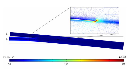
The 4PB technique was simulated using the finite element method. The geometry used for the
experiment has been reproduced in two-dimensional simulations. Due to the symmetry
conditions in the 4PB test, it is sufficient to consider only half of the structure as depicted in
Figure 4.27. All the materials are assumed to be linear elastic. On the left side of the
Figure 4.27 a symmetry condition was applied and a fixed point and a load point were applied
as in the experiment. Near the crack tip, a very fine triangular mesh was used. The initial
conditions for the simulations include an interface crack with a length of 1 mm, which has been
increased by 1 mm steps during the simulation until the desired value is reached.
In Figure 4.27 the results of a simulation with a=5 mm are shown. Due to the boundary
condition the Von Mises Stress is mainly generated at the h2 layer.
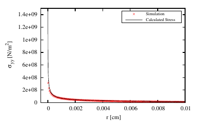
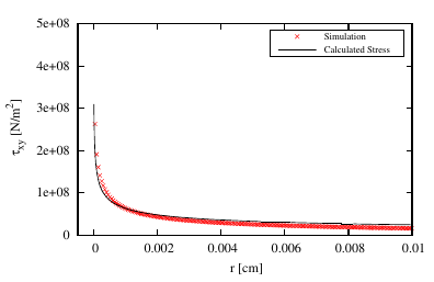
The stress distribution at the interface crack opening is described by (4.37). For every
crack length the σyy and τxy values were extracted as a function of r. Figure 4.28
and Figure 4.29 show an example of the obtained results, where the cross dots are
the values of the stresses obtained from the FEM simulations. The x-axis indicates
the interface distance at the right side of the crack-tip (r) and the y-axis the stress
value. Here, the singularity described in Section 4.1.2 can be observed for both
stresses.
The simulation results are obtained by using the approach described in Section 4.3.2 where the
values of σyy and τxy were extracted from the FEM simulations. The G values are calculated by
applying the approach for every simulated crack length in the range from 1 mm to 10
mm.
In Figure 4.28 and Figure 4.29 the results of the regression analysis are compared with
the FEM simulation results. By using the approach described in Section 4.3.2 the values of K1
and K2 were obtained; by subsequently inserting them in (4.40) the stresses at the interface can
be reproduced. The reproduced stresses qualitatively and quantitatively match the FEM
simulation results very closely.
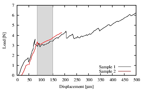
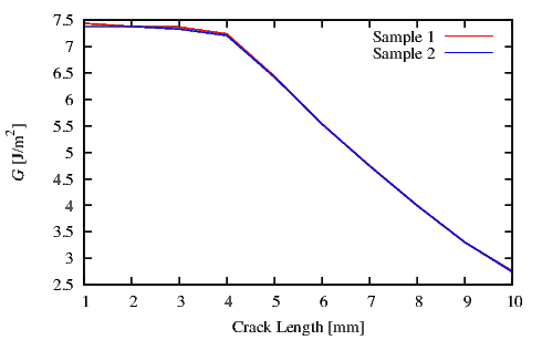
Figure 4.30 displays the G values calculated at every crack length a for the Sample 1
and Sample 2 (Table 4.4). As the crack approaches the fixed point of the 4PB test
(4 mm from the center of the samples, m in Figure 4.24) the G value decreases [88].
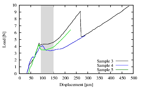
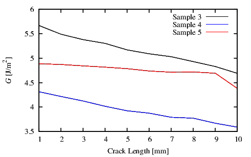
The simulated value G at every crack length a for Sample 3, Sample 4, and Sample 5
(Table 4.4) is shown in Figure 4.31. Here the decrease in G is less pronounced than in
Sample 1 and Sample 2. The value m=10 mm (same as in the experiment) was used and
the simulations were executed until the crack length of a=10 mm was reached. The
different line slopes are due to the different thicknesses and interfaces of the analyzed
sample.
The experimental Gc was determined by using the average of the loads in a steady state
range. In addition, for the FEM simulation results an average value for Gc was determined. In
particular for Sample 1 and Sample 2 Gc was calculated in a range of crack lengths from 1 mm
to 4 mm and for Sample 3, Sample 4 and Sample 5 in a range of crack lengths from 3 mm to
9 mm.
|
|
|
|
| Sample | Experimental Gc[J∕m2] | Simulation Gc[J∕m2] | % Error |
|
|
|
|
| 1 | 5.95 | 7.36 | 19,2 |
| 2 | 5.9 | 7.33 | 19,5 |
| 3 | 4.6 | 5.10 | 9,8 |
| 4 | 3.5 | 3.88 | 9,8 |
| 5 | 3.9 | 4.75 | 17,9 |
|
|
|
|
| |
Table 4.5: Gc values measured from experimental data and calculated using FEM
simulations. The Gc values calculated for Sample 3, Sample 4, and 5 are in good agreement
with the experimentally measured Gc values.
In Table 4.5 the Gc values obtained from experimental and simulation data are
compared. For Samples 1 and 2 the FEM simulation results differ from the experiments
results. This difference is attributed to the behavior observed in Figure 4.25. In these
load-displacement plots no clean steady state regions can be observed. The discontinuous
sections of the load plots are a result of an unstable crack propagation. It is quite possible
that due to some defects or imperfect adhesion between the layers the delamination
propagates unevenly. This is also understandable considering the percent of delamination in
these two samples (cf. Table 4.4). For Sample 1 and Sample 2 the percentage of
delamination is 28 % and 7 %, respectively. For Sample 3, Sample 4, and Sample 5 the
percentage of delamination is over 75 % that indicates a stable crack propagation.
The FEM simulation results for Sample 3, Sample 4, and Sample 5 appear closer, as
given in Table 4.5. The Gc values for Sample 3 and Sample 4 are very close to the
experimental values. This is again due to a better adhesion in a longer region and thus a
more pronounced steady state load area. In Figure 4.26 a distinguishable constant
load created as a result of the delamination is observed. The FEM simulation results
the Sample 5 is less accurate but still in an acceptable range (cf. % Err. in Table
4.5).
Simulation results and experimental data imply that the influence of the additional Ti layer
(Table 4.4) is negligible.
A FEM simulation method to calculate the energy release rate G at the interface between
two materials was presented. The 4PB technique can be simulated by considering
a simplified structure. From the FEM simulations, the stress at the interface was
obtained and used to calculate the energy release rate G. The results of FEM simulations
strongly depend on the quality of the experimental data. For the calculation of Gc it is
necessary to start with a load-displacement plot, where a steady state load is clearly
observable and distinguishable. This study demonstrated the efficiency of the FEM
simulation and how it can be used to calculate G for different boundary conditions and
geometries of the TSV structure, where the delamination is a potential reliability
issue.
The results obtained are in good agreement with experimental measurements. Therefore, the
developed model provides a convenient tool for the study of delamination issues in
TSVs.
In the previous sections two different methods for the calculation of the energy release rate G
were presented, namely J-Integral and regression analysis. The results in Section 4.5 show
good agreement between experimental data and simulations. Therefore, the developed method
correctly represent the physical delamination behavior.
A comparison between the two methods is given in this section. Using an identical structure
G was calculated with the two methods. The results of the two methods are compared to verify
their quality with respect to the G value.
Figure 4.32 depicts the structure under simulation. At the left side of the structure a
symmetric condition was set. Layer 1 indicates Si and layer 2 indicates SiO2 films. Si has a
thickness of 70 μm and SiO2 of 72.6 μm. The length w was set to 2.22 mm and the applied
force F has a value of 0.2 N. The fixed point was positioned at m=1 mm from the left side of
the structure.
As used previously in the other simulations also here a stationary simulation was performed.
Crack lengths in the range from 0.1 mm to 0.9 mm were simulated.
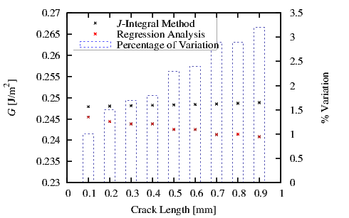
In Figure 4.33 the simulation results are presented. There is a clear agreement between the
two methods. The black crosses indicate the results obtained from the J-Integral method and
the red crosses are the results obtained from the regression analysis. Both methods give a
constant G for every simulated crack length.
The two methods were verified for the same structure. The results are effectively identical.
As shown in Figure 4.33 the variation in percentage between the two methods varies
from 1% at small crack lenghts to 3.2% at long crack lengths. The regression analysis
becomes less accurate as the simulated crack lengths approach the fixed point m of the
structure [87]. The J-Integral method is implemented in a FEM tool. This method permits to
calculate the G value directly at the end of the simulation. The method needs to
calculate an integral over a path between the two materials. If the material thickness of
one layer or both is too thin, the inability of defining a path for the integral can be
encountered.
The regression analysis can be applied when thin films are taken in account. It produces the
same results, but the evaluation time necessary to calculate G is higher, as the results have to be
post processed. After the simulation, the stress at the interface needs to be collected and
used in a statistical analysis software, which is used to perform the post-processing
fitting.
In this chapter the delamination theory was explained and the probability of delamination at
several material interfaces, essential for the fabrication of an open TSV was investigated.
The energy release rate G, which is an important measure for delamination prediction, was
calculated at different interfaces. By comparing G with the critical energy release rate Gc
predictions about the probability of delamination can be made. Two different methods used in
calculations of G were implemented using FEM. The J-Integral method permits to
obtain G at the end of the FEM simulation. The regression analysis method, however
requires two post-processing steps. In the first step the obtained stress values at the
interface between the two materials need to be extracted. In the second step, through a
regression analysis of the collected stress values K1 and K2, necessary to calculate G are
determined.
The second method was verified by replicating experiments and the obtained results
sufficiently reproduce the measured results. Therefore, the two methods were employed to
calculate G for the same structure. The results obtained from the two methods are in good
agreement.
While investigating the material interfaces present in open TSVs using the J-Integral
method, it was found that the most critical conditions were at the SiO2/W interface. For this
interface the Gc was determined experimentally (Section 4.5) and the simulated value
(3.5-5.95 J/m2) was higher than that found in literature (0.2-0.5 J/m2 [84]). This difference is
caused by a particular configuration of the film/substrate geometry. The thickness of the layers,
the residual stress of the layers, and the employed method to calculate Gc produce different
results. Open TSVs have sophisticated structures which do not permit to know the
critical condition for the failure. Therefore we are able to qualitatively predict the most
unstable condition for delamination by comparing G with the lowest Gc found in
literature.
The SiO2/W interface is fundamental for the mechanical stability of open TSVs. G was
calculated by investigating the influence of factors such as residual stresses in the films,
thicknesses of the layers and, force applied to the system. It was determined, that the most
unstable system is one where the residual stress in the W layer is very high, a high external force
is applied, or the W film is very thin. Therefore, in the next chapter the origin of the residual
stress in solid films is studied.