|
|
|
|
Previous: B.3 HEISENBERG Picture Up: B. Time Evolution Pictures Next: B.5 Imaginary Time Operators |
|
|
|
|
Previous: B.3 HEISENBERG Picture Up: B. Time Evolution Pictures Next: B.5 Imaginary Time Operators |
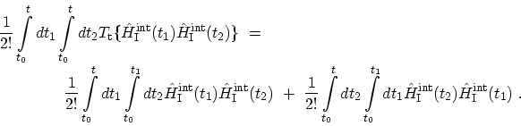 |
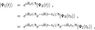
(B.22) |
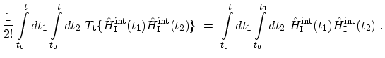 |
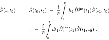
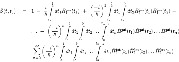
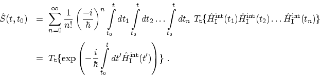
(B.23) |
|
|
|
|
Previous: B.3 HEISENBERG Picture Up: B. Time Evolution Pictures Next: B.5 Imaginary Time Operators |