C. Review of Thermodynamics and Statistical Mechanics

The fundamental thermodynamic identity

$$\begin{array}{l}\displaystyle dE \ = \ TdS \ - PdV \ + \ E_\mathrm{F} dN \ , \end{array}$$ (C.1)

specifies the change in the internal energy $E$ arising from small independent changes in the entropy $S$, the volume $V$, and the number of particles $N$. Equation (C.1) shows that the internal energy is a function of these three variables, $E=E(S,V,N)$, and that the temperature $T$, the pressure $P$, and the FERMI energy $E_\mathrm{F}$ (also called the chemical potential) are related to the partial derivatives of $E$

$$\begin{array}{l}\displaystyle T \ = \ \left(\frac{\partial E}... ... \left(\frac{\partial E}{\partial N}\right)_{SV}\ . \end{array}$$ (C.2)

In practice, however, experiments are usually performed at fixed $T$ and it is convenient to make LEGENDRE transformation to the variables $(T,V,N)$ or $(T,P,N)$. The resulting functions are known as HELMHOLTZ free energy $F(T,V,N)$ and GIBBS free energy $G(T,P,N)$. It is often important to consider the set of independent variables $(T,V,E_\mathrm{F})$, which is appropriate for variable $N$. A further LEGENDRE transformation leads to the thermodynamic potential

$$\begin{array}{l}\displaystyle \Omega(T,V,E_\mathrm{F}) \ = \ ... ...thrm{F} N \ = \ E \ - \ TS \ - \ E_\mathrm{F} N \ , \end{array}$$ (C.3)

with the corresponding differential and coefficients

$$\begin{array}{l}\displaystyle d\Omega(T,V,E_\mathrm{F}) \ = \ - \ SdT \ - \ PdV \ - N dE_\mathrm{F} \ , \end{array}$$ (C.4)

$$\begin{array}{l}\displaystyle S \ = \ -\left(\frac{\partial\O... ...artial\Omega}{\partial E_\mathrm{F}}\right)_{TV}\ . \end{array}$$ (C.5)

Although $E$, $F$, $G$, and $\Omega$ represent equivalent ways of describing the same system, their natural independent variables differ in one important way. In particular, the set $(S,V,N)$ consists entirely of extensive variables, proportional to the actual amount of matter present. The transformation to $F$ and then to $G$ or $\Omega$ may be interpreted as reducing the number of extensive variables in favor of intensive ones that are independent of the total amount of matter.

To this point, only macroscopic thermodynamics has been discussed. The microscopic content of the theory must be added separately through statistical mechanics, which relates the thermodynamic functions to the HAMILTONian of the many-particle system. The elementary discussions of statistical mechanics usually consider systems containing a fixed number of particles. This approach, which is refereed to as canonical ensemble, is too restricted for our purposes. 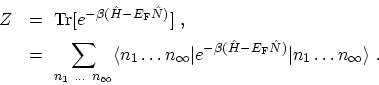To include the possibility of a variable number of particles the grand canonical ensemble can be employed. For a grand canonical ensemble at FERMI energy $E_\mathrm{F}$ and temperature $T$, the grand partition function $Z$ is defined as

$$\begin{array}{ll} Z\ &\displaystyle \equiv \ \sum_{N} \sum_{i... ...{Tr}[e^{-\beta(\hat{H}- E_\mathrm{F} \hat{N})}] \ , \end{array}$$ (C.6)

where $i$ denotes the set of all states for a fixed number of particles $N$, and the sum implied in the trace is over both $i$ and $N$. Short-hand notation $\beta=1/k_\mathrm{B}T$ has been introduced, where $k_\mathrm{B}$ is the BOLTZMANN constant. A fundamental result from statistical mechanics states that

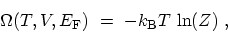$$\begin{array}{l}\displaystyle \Omega(T,V, E_\mathrm{F}) \ = \ - k_\mathrm{B}T\ \mathrm{ln}(Z) \ , \end{array}$$ (C.7)

which allows one to compute all the macroscopic equilibrium thermodynamics from the grand partition function. The statistical operator $\rho$ corresponding to (C.6) is given by

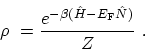$$\begin{array}{l}\displaystyle \rho\ = \frac{e^{-\beta(\hat{H}- E_\mathrm{F} \hat{N})}}{Z} \ . \end{array}$$ (C.8)

For any operator $\hat{O}$, the ensemble average $\langle \hat{O} \rangle$ is achieved with the prescription

$$\begin{array}{ll}\displaystyle \langle \hat{O}\rangle \ &\dis... ...Tr}[e^{-\beta(\hat{H}- E_\mathrm{F} \hat{N})}]} \ . \end{array}$$ (C.9)

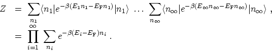
By applying these results the properties of a gas of non-interacting Bosons or FERMIons can be studied. If (C.6) is written out in detail with the complete set of states in the abstract occupation number HILBERT space, one gets

$$\begin{array}{ll}\displaystyle Z\ &\displaystyle = \ \mathrm{... ...rm{F} \hat{N})}\vert n_1\ldots n_\infty \rangle \ . \end{array}$$ (C.10)

Since these states are eigen-states of the non-interacting HAMILTONian $\hat{H}_{0}$ and the number operator $\hat{N}$, both operators can be replaced by their eigen-values

$$\begin{array}{ll}\displaystyle Z\ &\displaystyle = \ \sum_{n_... ...\right)\right] \vert n_1\ldots n_\infty \rangle \ . \end{array}$$ (C.11)

The exponential is now a number and is equivalent to a product of exponentials. Therefore, the sum over expectation values factor into a product of traces

$$\begin{array}{ll}\displaystyle Z\ &\displaystyle = \ \sum_{n_... ...sum_{n_i} e^{-\beta(E_{i}- E_\mathrm{F} )n_{i}} \ . \end{array}$$ (C.12)

M. Pourfath: Numerical Study of Quantum Transport in Carbon Nanotube-Based Transistors