4.4 Mode-Space Transformation

A mode space approach significantly reduces the size of the HAMILTONian matrix [9]. Due to quantum confinement along the CNT circumference, circumferential modes appear and transport can be described in terms of these modes. If $M$ modes contribute to transports, and if $M<n$, then the size of the problem is reduced from $n\times N$ to $M \times N$, where $N$ is number of carbon rings along the CNT. If the potential profile does not vary sharply along the CNT, subbands are decoupled [9] and one can solve $M$ one-dimensional problems of size $N$.

Mathematically, one performs a basis transformation on the HAMILTONian of the $(n,0)$ zigzag CNT to decouple the problem into $n$ one-dimensional mode space lattices [243]

$$\begin{array}{ll} \ensuremath{{\underline{H}}}^{'} \ &\displa... ...] & & & & \bullet & \bullet \end{array} \right]} \ ,\end{array}$$ (4.20)

with

$$\begin{array}{lll} \ensuremath{{\underline{U}}}^{'}_i & \disp... ...\underline{t}}}_2 \ \ensuremath{{\underline{S}}}\ , \end{array}$$ (4.21)

where $\ensuremath{{\underline{S}}}$ is the transformation matrix from the real space basis to the mode space basis. The purpose is to decouple the modes after the basis transformation, i.e., to make the HAMILTONian matrix blocks between different modes equal to zero. This requires that after the transformation, the matrices $\ensuremath{{\underline{U}}}_i$, $\ensuremath{{\underline{t}}}_1$, and $\ensuremath{{\underline{t}}}_2$, become diagonal. Since $\ensuremath{{\underline{U}}}_i$ and $\ensuremath{{\underline{t}}}_1$ are identity matrices multiplied by a constant, they remain unchanged and diagonal after any basis transformation, $\ensuremath{{\underline{U}}}^{'}_i=\ensuremath{{\underline{U}}}_i$ and $\ensuremath{{\underline{t}}}^{'}_1 = \ensuremath{{\underline{t}}}_1$. To diagonalize $\ensuremath{{\underline{t}}}_2$, elements of the transformation matrix $\ensuremath{{\underline{S}}}$ have to be the eigen-vectors of $\ensuremath{{\underline{t}}}_2$. These eigen-vectors are plane waves with wave-vectors satisfying the periodic boundary condition around the CNT. The eigen-values are

$$t^\nu_2\ =\ 2te^{-i\pi\nu/n}\cos(\pi\nu/n) \ ,$$ (4.22)

where $\nu=1,2,\ldots,n$ [243]. The phase factor in (4.22) has no effect on the results such as charge and current density, thus it can be omitted and $t^\nu_2\ =\ 2t\cos(\pi\nu/n)$ can be used instead.

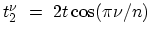
Figure 4.7: Zigzag CNT and the corresponding one-dimensional chain with two sites per unit cell with hopping parameters $t$ and $t^\nu_2\ =\ 2t\cos(\pi\nu/n)$.

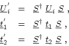
After the basis transformation all sub-matrices, $\ensuremath{{\underline{U}}}_i$, $\ensuremath{{\underline{t}}}_1$, and $\ensuremath{{\underline{t}}}_2$ are diagonal. By reordering the basis according to the modes, the HAMILTONian matrix takes the form

$$\ensuremath{{\underline{H}}}^{'} \ = \ { \left[ \begin{array}{ccc... ...h{{\underline{H}}}^\nu & & \\ [1.5pt] & & & & \bullet & \end{array} \right]}\ ,$$ (4.23)

where $\ensuremath{{\underline{H}}}^\nu$ is the HAMILTONian matrix for the $\nu$th mode [243]

$$\ensuremath{{\underline{H}}}^\nu = { \left[ \begin{array}{cccccc}... ...\\ & & & t & U_5 & \bullet\\ & & & & \bullet & \bullet \end{array} \right]} \ .$$ (4.24)

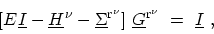
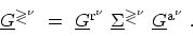
The one-dimensional tight-binding HAMILTONian $H^\nu$ describes a chain of atoms with two sites per unit cell and on-site potential $U$ and hopping parameters $t$ and $t^\nu_2$ (Fig. 4.7). The spatial grid used for device simulation corresponds to the circumferential rings of carbon atoms. Therefore, the rank of the matrices for each subband are equal to the total number of these rings $N$. Self-energies can be also transformed into mode space $\Sigma^\nu$, see Section 4.5 and Section 4.6. The GREEN's functions can therefore be defined for each subband (mode) and one can solve the system of transport equations for each subband independently

$$\begin{array}{l} [E \ensuremath{{\underline{I}}} - \ensuremat... ...athrm{r^\nu} \ = \ \ensuremath{{\underline{I}}} \ , \end{array}$$ (4.25)

$$\begin{array}{l} \ensuremath{{\underline{G}}}^{\gtrless^\nu} ... ...} \ \ensuremath{{\underline{G}}}^\mathrm{a^\nu} \ . \end{array}$$ (4.26)

M. Pourfath: Numerical Study of Quantum Transport in Carbon Nanotube-Based Transistors