4.4.1 Volume Models

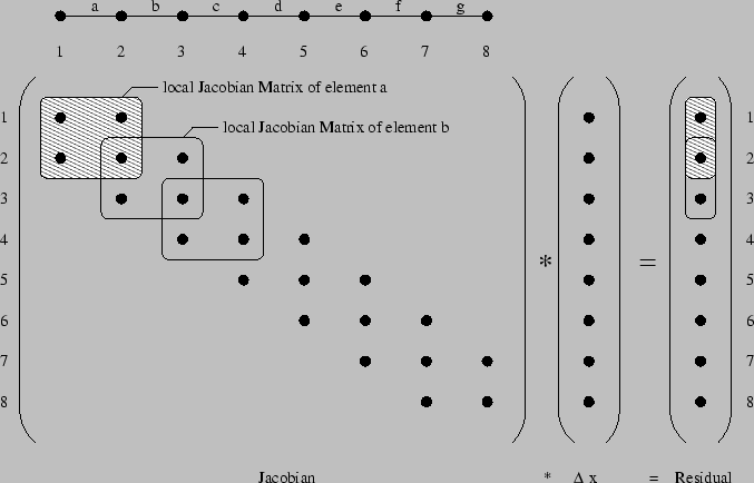
A lot of partial differential equations can be discretized so that finally a sparse matrix results which represents a linear equation system that has to be solved (Fig. 4.9). In case of non linearity an iteration is necessary where successive approximations are calculated. The condition for the nonlinear system

f (x_s) = 0 (4.6)

is satisfied in case of

$$\left(\vphantom{x_i }\right. \left.\vphantom{x_i }\right)$$ (4.7)

Looking at the first order of the Taylor series

$${\frac{\partial f(x_i)}{\partial x_i}} \left(\vphantom{ x_s - x_i }\right. \left.\vphantom{ x_s - x_i }\right) \left(\vphantom{ x_s - x_i }\right. \left.\vphantom{x_s - x_i }\right)^{2}_{}$$ (4.8)

it is obvious that in case of a linear approximation where terms of higher order are neglected ( O$\left(\vphantom{x_s - x_i }\right.$x_s - x_i$\left.\vphantom{x_s - x_i }\right)^{2}_{}$ = 0) the resulting linear equation system

$$\Delta$$ (4.9)

satisfies the postulated condition when R $\rightarrow$ 0. In case of linear systems the solution can immediately be determined by

$$\Delta$$ (4.10)

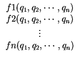
The vector f(x) denotes the so called Residual function

$$\left(\vphantom{ \begin{array}{c} f1(q_1,q_2,\cdots,q_n)\\ f2(q_1,q_2,\cdots,q_n)\\ \vdots \\ fn(q_1,q_2,\cdots,q_n) \end{array}}\right. \begin{array}{c} f1(q_1,q_2,\cdots,q_n)\\ f2(q_1,q_2,\cdots,q_n)\\ \vdots \\ fn(q_1,q_2,\cdots,q_n) \end{array} \left.\vphantom{ \begin{array}{c} f1(q_1,q_2,\cdots,q_n)\\ f2(q_1,q_2,\cdots,q_n)\\ \vdots \\ fn(q_1,q_2,\cdots,q_n) \end{array}}\right)$$ (4.11)

which is a vector of functions of the searched quantities q₁, q₂, ^... , q_n. Its derivative stands for the system matrix or also called Jacobian Matrix and can be calculated using the following rule

$$\left(\vphantom{ \begin{array}{cccc} \frac{\partial f1(q_1,q_2,\h... ...dots & \frac{\partial fn(q_1,q_2,\cdots,q_n)}{\partial q_n} \end{array}}\right. \begin{array}{cccc} \frac{\partial f1(q_1,q_2,\hdots,q_n)}{\parti... ..._2} & \cdots & \frac{\partial fn(q_1,q_2,\cdots,q_n)}{\partial q_n} \end{array} \left.\vphantom{ \begin{array}{cccc} \frac{\partial f1(q_1,q_2,\h... ...dots & \frac{\partial fn(q_1,q_2,\cdots,q_n)}{\partial q_n} \end{array}}\right)$$ (4.12)

AMIGOS uses this mathematical expression profitably so that an automatic assembling of the global stiffness matrix is done depending on the basis of a discretized simulation domain. It simplifies the task of global assembling of all grid points and reduces it to a local process where the PDE system has to be discretized only on a single element. To preserve one's survey it is much easier to handle just the smaller local part of the discretization than dealing with the global assembling step (Fig. 4.9). Furthermore, AMIGOS releases the model developer from the duty to calculate the Jacobian matrix using its derivative operator that derives the residual function symbolically.

Figure 4.9: Auto assembling mechanism of a one-dimensional simulation domain with linear two point elements