3.4.2 Diffuse Interface Model

The diffuse interface method, or phase field method, offers an attractive alternative to the sharp interface model for solving problems related to the electromigration evolution of the void surface. Various authors [108,107,10,11] have applied the diffuse interface approach to predict the motion and growth of voids in interconnects due to electromigration and stress-induced surface diffusion. It should be pointed out that the diffuse interface model is viewed as an approximation to the sharp interface model of Section 3.4.1.

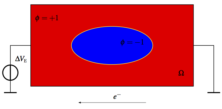
The interconnect line is idealized as a two-phase system consisting of the material "phase" and the void "phase". The introduction of a smooth order parameter field φ (or phase field variable) to describe the void structure circumvents the surface tracking used in the sharp interface method. The order parameter takes on constant values in the material phase (φ=+1) and in the void phase (φ=-1) in the entire domain Ω and changes rapidly from one to the other over a narrow interfacial layer which represents the void surface, as illustrated in (3.6). The basic concept of the diffuse interface approach involves the spread of the sharp metal/void interface into a narrow interfacial layer between the metal phase and the void phase. In the limit of vanishing interface layer thickness, the two models will perfectly match.

Figure 3.6: Order parameter distribution in a 2D conducting metal line.

The form of the equations governing the dynamics of the order parameter is based on the microforce balance principle of Gurtin [72]. Inhomogeneous systems involve domains of well-defined phases separated by a narrow interface ((3.6)). If the phases are driven out of equilibrium, one phase will grow at the cost of the other. Thermodynamic equilibrium is reached if the state of a system remains constant [53]. Therefore, the system tends to move towards the equilibrium condition. During this transition, the free energy of the system is minimized. The minimization of the free energy rate yields the dynamics equations governing the evolution of the near-equilibrium system [130]. Diffuse interface models are introduced to study systems out of equilibrium. Traditional diffuse interface models are connected to thermodynamics by a phenomenological free energy functional written in terms of the order parameter, its gradient, and the local strain. The free energy functional F, which divides the entire domain Ω in (3.6) into two regions of constant order parameter value separated by a narrow metal-void interface [107], is chosen as

\[\begin{equation} F(\phi,\nabla\phi,\overline{\overline\epsilon})=\int_{\Omega} \left[\cfrac{2 \gamma_\text{s}}{\epsilon_\text{di} \pi}\left(\frac{1}{4}(\phi^2-1) ^2 + \frac{1}{2}\epsilon_\text{di}^2 |\nabla\phi|^2 \right)+\cfrac{\overline{\overline\sigma} : \overline{\overline\epsilon}}{2}\right] \,\text{d}\Omega, \end{equation}\] (3.78)

where γ_s is the isotropic surface energy and ε_di is the parameter which scales with the thickness of the interface located at the void surface. For reasons mentioned in the previous section, the effect of the elastic strain energy on the free energy functional is neglected, when it comes to the analysis of the void evolution mechanism for passivated copper lines. For simplicity, both surface energy and surface diffusivity are assumed to be isotropic.

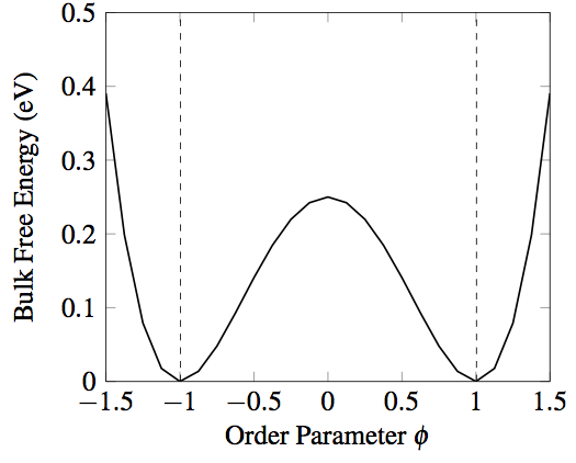
The two terms in round brackets in the free energy functional equation (3.78) describe the surface free energy. The surface free energy represents the energy cost associated with the addition or removal of material from the void surface [130]. The first surface free energy term in equation (3.78) is related to the bulk free energy. Conventionally, it is taken to be a quartic double well potential [107] which drives phase separation, with two minima corresponding to the material and the void phases. Bhate [11,10] employed an alternative form of the bulk free energy function based on the double obstacle potential proposed by Oono [119]. By choosing a bi-quadratic function, order parameter solutions different from +1 and -1 are penalized, as shown in (3.7).

Figure 3.7: Quartic double well potential for the free energy function.

The presence of the bulk free energy term, as a bi-quadratic function, in the free energy functional equation (3.78) requires the order parameter to be computed throughout the bulk of the line, not only within the narrow interfacial layer marking the void surface. The second surface free energy term in equation (3.78) represents the gradient energy (or interfacial energy), which denotes the contribution of the diffuse interface [53]. The void interface is located at those sites in the domain with nonzero gradients. As a result, the order parameter is defined in such a way that the volume fractions of the material and void phases are 1+φ/2 and 1-φ/2, respectively. Significant deviations of the order parameter from either +1 or -1 occur only within the metal-void interface.

The free energy functional provides an expression for the chemical potential μ_s of an atom in the interfacial region, which is the functional derivative of the free energy functional with respect to the order parameter function, and is given by

\[\begin{equation}\begin{split} \mu_\text{s}&= 2 \Omega_\text{a} \frac{\delta{\mathscr{F}}}{\delta\phi} =2 \Omega_\text{a} \left(\cfrac{\partial \mathscr{F}}{\partial \phi}- \nabla \cdot \left(\cfrac{\partial \mathscr{F}}{\partial \nabla\phi}\right)\right)\\ &=\cfrac{4 \gamma_\text{s}\Omega_\text{a}}{\epsilon_\text{di} \pi}\left(\phi(\phi^2-1)-\epsilon^2_\text{di} \nabla^2\phi \right). \end{split} \end{equation}\] (3.79)

The factor of 2 multiplying Ω_a in the chemical potential equation is introduced as the order parameter transition from +1 in the material to -1 in the void across a narrow interface [11]. As described above, the elastic strain energy term of equation (3.78) is not considered in the further development of the model.

The chemical potential relates to the driving force of diffusion F_d=-∇μ_s. In fact, as discussed in Section 3.4.1, atoms diffuse on the void surface from high chemical potential regions to low chemical potential regions. In Section 3.2 it has been shown that the material transport responsible for electromigration failure occurs due to a combination of different driving forces, such as the electron wind, the mechanical stress gradient, and the temperature gradient. The electromigration force F_em is the most dominant driving force with regards to the mass flux responsible for electromigration-induced void evolution [118]. Stress and temperature gradients are therefore not taken into account as driving forces for mass transport [62]. Furthermore, the electromigration-induced material transport on the void surface is assumed to be faster than diffusion in the bulk of the metal line [71]. In the presence of electromigration the total driving force leads to the mass flux J_s along the void surface as

\[\begin{equation} \vec{J_\text{s}}=\cfrac{2 D_\text{s}(\phi)}{\epsilon_\text{di} \pi} \left(\vec{F_\text{d}}+\vec{F_\text{em}}\right)= -\cfrac{2 D_\text{s}(\phi)}{\epsilon_\text{di} \pi}\left(\nabla\mu_\text{s}-e|Z^*|\nabla V_\text{e}\right), \end{equation}\] (3.80)

In order to confine diffusion to the void surface only, the isotropic surface diffusivity function D_s(φ) is set to

\[\begin{align} D_\text{s}(\phi) = \begin{cases} \cfrac{D_\text{s} \delta_\text{s}}{k_\text{B}T} & \mbox{if } |\phi|\mbox{<1}, \\ 0 & \mbox{otherwise.} \mbox{} \end{cases} \end{align}\] (3.81)

Note that the function D_s(φ) vanishes outside the interfacial region [10]. Since the order parameter is a conserved quantity, its evolution can be described as a consequence of divergences in the surface flux by the following equation

\[\begin{align} \cfrac{\partial \phi}{\partial t} = -\ \nabla \cdot \vec{J_\text{s}} = \cfrac{2 D_\text{s}(\phi)}{\epsilon_\text{di} \pi}~\nabla \cdot\left(\nabla\mu_\text{s}-e|Z^*|\nabla V_\text{e}\right)+ \cfrac{2}{\epsilon_\text{di} \pi}~\nabla D_\text{s}(\phi) \cdot \left(\nabla\mu_\text{s}-e|Z^*|\nabla V_\text{e}\right). \end{align}\] (3.82)

This equation is the so-called Cahn-Hilliard equation [21,22], which is a 4th-order PDE with modifications due to the presence of an electrical potential gradient. Since ∇D_s(φ) is a distribution the second term on the right hand side of equation (3.82) is a flux term modeling inflow or outflow of atoms through the metal-void interface. The above equation (3.82) is supplemented with no-flux boundary conditions and initial values for the order parameter field in the entire domain Ω (3.6) as follows

\[\begin{align} \hat{n} \cdot \vec{J_\text{s}} = 0 \quad \text{on} \quad \Gamma_{ext},\\ \phi(x,0)=\phi^0(x)\in [-1,1]\quad \forall x\in\Omega, \end{align}\] (3.83-3.84)

where n is the outward normal vector at the surface. The no-flux boundary condition leads to the conservation of the void's area. In this way, the solution of φ in equation (3.82) possesses the properties that the total free energy of the metal-void system diminishes to maintain thermodynamic equilibrium and that the total mass is conserved. Further boundary conditions which relate void growth due to electromigration-driven diffusion to an appropriate case study are presented in detail in Chapter 5.

In addition, the evolution equation for the order parameter which describes the void's change in shape or the void's drift along the metal line must be related to the equation determining the electric current induced mass transport in the metal line. As discussed in Section 3.1, the electric potential at any point in the interconnect is related to the electric current density j by Ohm{'}s law

\[\begin{equation} \vec{j} = - \sigma_\text{e}(\phi)\nabla V_\text{e}, \end{equation}\] (3.85)

where σ_e is the electrical conductivity of the metal. In this way, the current density distribution can be evaluated in the entire domain. In the sharp interface model, the void surface acts as an insulating boundary for the electric current flowing through the line. In order to incorporate the no current flux boundary condition at the void surface in the diffuse interface model [10], the electrical conductivity is chosen to vary as the order parameter goes from +1 in the material to -1 in the void by

\[\begin{equation} \sigma_\text{e}(\phi)= \cfrac{\sigma_\text{e}^\star}{2}\left(\phi+1\right). \end{equation}\] (3.86)

This simple linear function reduces conductivity to its bulk value σ_e^* in the metal "phase", but vanishes within the void "phase". For small values of the ε_di parameter this condition ensures an appropriate boundary condition at the void surface. As described previously, the evolution of the void is due mainly to material transport at the void surface, driven by the electromigration force. The mass flux J_s along a void surface is assumed to be proportional to the component of the current density tangential to the surface j_es. By assuming a zero normal current density at the void surface, the tangential current density j_es is described as the average current density over the void surface [28] given by

\[\begin{equation} {j_\text{es}} = 2 \cfrac{\int_{\Omega} ||{\vec{j}}|| (1-\phi^2) \text{d}\Omega}{\int_{\Omega} (1-\phi^2) \text{d}\Omega}, \end{equation}\] (3.87)

where the term 1-φ² is non-zero only at the void-metal interface. Equations (3.85) and (3.87) allow one to determine the current density distributions in the metal-void system and at the void surface, respectively. Since electric charge should be conserved, the distribution of electric potential in the line is determined by the Laplace equation

\[\begin{equation} \nabla \cdot \left(\sigma_\text{e}(\phi)\nabla V_\text{e}\right) = 0. \end{equation}\] (3.88)

The order parameter distribution in the line is therefore determined for each time step by coupling the solutions of the dynamic equation of the order parameter (3.82) together with the solutions of the electrical problem (equations (3.85)-(3.88)).

The capabilities of the diffuse interface model are validated by performing two convenient tests of numerical accuracy on a simple 2D rectangular metal line, in order to evaluate the different impacts of surface energy and electromigration on the diffusion underlying the evolution of the void in the interconnect. First, the evolution of a non-circular void towards its equilibrium shape is examined, in the absence of any electrical potential gradient in the metal line. Simulations are performed using the diffuse interface model.

Figure 3.8: Evolution of an elliptical void in a non-electrically conducting line. The ellipse collapses into a circle due to surface energy driven diffusion.

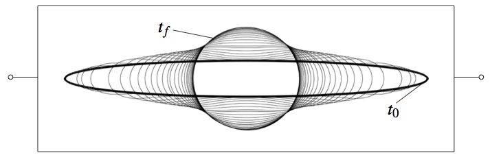The results, depicted in (3.8), represent the zero contours of the order parameter at different time steps. Under conditions of surface energy driven diffusion, the system tends to minimize the surface free energy by minimizing the void surface. As a result, the elliptical void is expected to relax to a circular void in time [11], which is exactly what the simulation shows.

Next, the migration of a circular void in a rectangular metal interconnect, subjected to an electromigration force, is analyzed by tracking the order parameter distribution in the structure. The electromigration effect is induced in the line by applying a voltage ΔV_e across its ends ((3.9)).

Figure 3.9: Order parameter distribution of an evolving stable circular void in an interconnect line under electrical loading ΔV_e. The void profiles are plotted at (a) t = 0s, (b) t = 1s, (c) t = 2s, and (d) t = 20s. The void maintains its circular shape as it migrates through the line due to a combination of the surface energy gradient and the electromigration force.

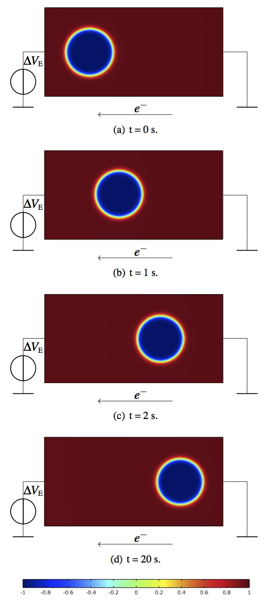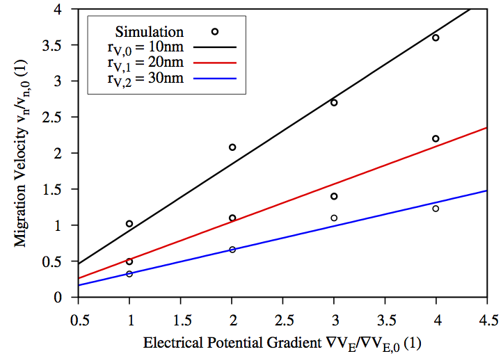
In this case, the resulting void evolution is a consequence of a complex coupling of driving factors: migration due to the electromigration force counteracted by a predisposition towards minimizing the surface of the void [11]. (3.9) shows the typical numerical test results at different time steps. The void surface remains morphologically stable and the void moves towards the cathode at a constant velocity due to the electrical potential gradient, without undergoing additional changes in shape. This behavior is in accordance with the analysis of Ho [78], who has demonstrated that the evolving void maintains a stable circular shape and that the migration velocity v_n is linearly proportional to the applied electrical potential gradient ∇V_e and inversely proportional to the void radius r_v as follows

\[\begin{equation} v_\text{n}=2\cfrac{D_\text{s}\delta_\text{s}}{r_\text{v} k_\text{b}T}Z^*e\nabla V_\text{e}. \end{equation}\] (3.89)

In order to demonstrate the proportionality, the migration velocity is calculated by increasing the applied voltage ΔV_e in the line at different void radii, as illustrated in (3.10). The fit of the curves to equation (3.89) indicates that the velocities obtained from the simulations are in good agreement with the solution provided by Ho [78]. As expected, the numerical tests demonstrate the accuracy of the diffuse interface model within the limit as the interface width vanishes.

Figure 3.10: Migration velocity v_n as a function of electrical potential gradient for different void radii r_v. The lines indicate the fit according to equation (3.89).