

Next: 9.3.6 Simulation Results
Up: 9.3 Inverse Modeling of
Previous: 9.3.4 Handling Multiple Devices
Having this comprehensive model (Figure 9.7)
which delivers match metrics associated to a set of doping profile
parameters for each of our measured operating points, we are able to
perform the actual inverse modeling procedure using SIESTA's
optimization environment. Therefore, we define the optimization
experiment based on LMMIN as shown in
Example 9.6.

In this experiment description we define n3,
ysigma3, n4, and ysigma4 as free parameters
of the optimization. Therefore, the optimization tool will search for
the shape and the peak concentration of the threshold adjust implant
and for the well doping of the measured devices.
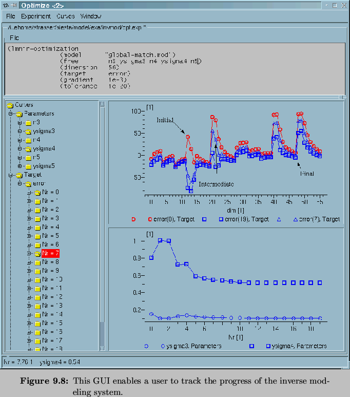
Figure 9.8 shows the inverse modeling procedure at
work. Plots display the match vector for each iteration, and for the
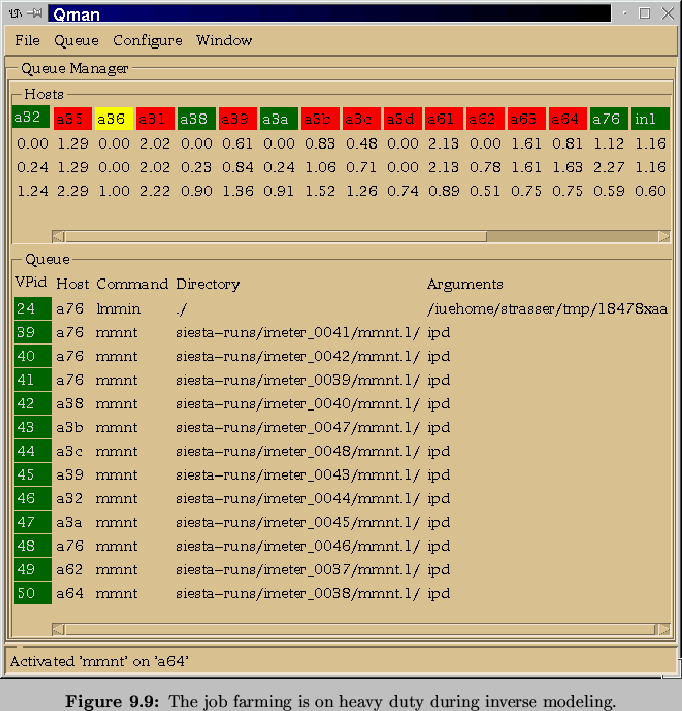
evolution of doping profile parameters. Figure 9.9 displays
the job farming system and as one can see from this screen shot,
computation hosts are utilized as far as possible. The user of this
system is able to produce Postscript files of all plots, which can be
displayed in the GUI, as it might be necessary for documentation
purposes.


Next: 9.3.6 Simulation Results
Up: 9.3 Inverse Modeling of
Previous: 9.3.4 Handling Multiple Devices
Rudi Strasser
1999-05-27

