Chapter 1
Introduction
With the continued shrinking of semiconductor devices, a deeper understanding of the underlying
physical processes is required in order to further improve device performance. Since it is
impossible to measure all details of carrier transport on the nanometer scale, the availability of
accurate theoretical descriptions is essential in order to gain insight into the physical processes by
means of numerical simulations. This so-called Technology Computer Aided Design (TCAD) has
become an indispensable ingredient for the development of faster, smaller and more
power-efficient devices.
Quantum effects have long been negligible for charge transport, but they gain importance
with each technology generation. Nevertheless, quantum effects are not considered further within
this thesis, even though the theory of carrier scattering is based on a quantum mechanical
foundation [67].
1.1 Semiclassical Carrier Transport
The Boltzmann Transport Equation (BTE) is commonly considered to provide the best
semiclassical description of carrier transport. Carriers are described in a classical fashion by a
continuous distribution function  , which depends on the spatial location
  , momentum
  and time
  . The carrier momentum
  is related to a quantum-mechanical wave
number
is related to a quantum-mechanical wave
number  by the relation
  , where
  is the modified Planck constant. Without
going into the details of various derivations (see e.g. [67, 68, 50]), the BTE is given
by
is the modified Planck constant. Without
going into the details of various derivations (see e.g. [67, 68, 50]), the BTE is given
by
 where function arguments are omitted. Here,
  denotes the carrier velocity in dependence of the
carrier momentum,
denotes the carrier velocity in dependence of the
carrier momentum,  refers to the electrostatic force, and
  is the scattering operator. A
formulation based on the wavevector
is the scattering operator. A
formulation based on the wavevector  rather than momentum
  transforms the gradient as
 .
.
The description of carries by means of a distribution function with respect to the spatial
variable  , the momentum
  and time
  leads to a seven-dimensional problem space, which
makes the direct solution of the BTE very demanding. As a consequence, simpler macroscopic
models have been derived from moments of the BTE. Most noteworthy in this regard are the
drift-diffusion equations presented in Sec. 1.1.1, which are obtained from the zeroth and first
moment of the BTE.
leads to a seven-dimensional problem space, which
makes the direct solution of the BTE very demanding. As a consequence, simpler macroscopic
models have been derived from moments of the BTE. Most noteworthy in this regard are the
drift-diffusion equations presented in Sec. 1.1.1, which are obtained from the zeroth and first
moment of the BTE.
While the drift-diffusion equations have been successfully employed throughout the 20th
century for TCAD, the characteristic lengths of modern devices are well outside the range of
validity of the model. Hence, even though variants of the drift-diffusion equations are still in use
for the simulation of recent device generations, their accuracy is highly questionable and
leads to poor results already in the linear regime [51]. More accurate macroscopic
transport models have been derived based on higher moments of the Boltzmann Transport
Equation (BTE). The energy transport model and the hydrodynamic model are derived
from the first four moments of the BTE and presented in Sec. 1.1.3 and Sec. 1.1.2
respectively. In Sec. 1.1.4 a transport model based on the first six moments of the BTE is
discussed.
Despite the good results obtained from macroscopic models, which are derived from moments
of the BTE in the micron and sub-micron regime, the necessary approximations cease to hold in
the deca-nanometer regime. As a consequence, a full solution of the BTE is desired. Since direct
numerical methods are typically limited by memory constraints which stem from the resolution of
the high-dimensional simulation domain, the method of choice is usually the stochastic Monte
Carlo method, which is presented in Sec. 1.1.5.
It should be noted that each of the transport models presented in the following has to be
solved self-consistently with the Poisson equation. To this end, nonlinear iteration schemes such
as those detailed in Sec. 2.4 are typically employed. For the sake of brevity, self-consistency is not
further addressed in the following subsections.
1.1.1 The Drift-Diffusion Model
Taking the zeroth-order moment of the BTE (1.1) leads to
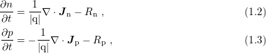 where
where  and
and  denote electron and hole densities and
  is the elementary
charge .
The recombination rates
is the elementary
charge .
The recombination rates  and
and  refer to Auger, radiative, and Shockley-Read-Hall
[95, 34] processes and can be expressed in terms of
refer to Auger, radiative, and Shockley-Read-Hall
[95, 34] processes and can be expressed in terms of  and
and  . Multiplication of the BTE with
the wave vector
. Multiplication of the BTE with
the wave vector  and integration over the
  -space leads to equations for the current densities
 and
and  :
:
 Carrier mobilities are denoted by
  and
and  , while
  and
and  are diffusion coefficients.
Substitution of (1.4) and (1.5) into (1.2) and (1.3) leads to a system of two partial differential
equations for the densities
are diffusion coefficients.
Substitution of (1.4) and (1.5) into (1.2) and (1.3) leads to a system of two partial differential
equations for the densities  and
and  . Equipped with suitable boundary conditions, these
equations completely specify the electron and hole densities. This so-called drift-diffusion model
was first derived by Van Roosbroeck in 1950 [103].
. Equipped with suitable boundary conditions, these
equations completely specify the electron and hole densities. This so-called drift-diffusion model
was first derived by Van Roosbroeck in 1950 [103].
As a prelude to numerical stabilization schemes discussed in Sec. 4.3, a direct discretization of
the drift-diffusion model by simple methods such as finite differences usually fails due to large
forces inside the device. Numerical stability for the drift-diffusion equations is increased
substantially by the use of upwind schemes in general, and the Scharfetter-Gummel scheme [90]
in particular. Additionally, a discretization is usually required to conserve current, hence box
integration schemes are commonly employed [93].
1.1.2 The Hydrodynamic Model
The consequence of taking the zeroth and the first moment of the BTE for the derivation of the
drift-diffusion model only is that a spatial dependence of average carrier energies are ignored. To
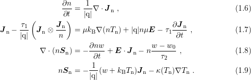
overcome these deficiencies, Bløtkjær derived conservation equations by taking the
zeroth, the first and the second moments of the BTE [5]. As closure condition for
the heat flux density  , Fourier’s law is applied, which leads for electrons to the
system
, Fourier’s law is applied, which leads for electrons to the
system
 The
model needs to be solved for the unknown electron density
The
model needs to be solved for the unknown electron density  , the electron temperature
 and the average energy
  . The contribution of the drift velocity to the carrier
energy is often neglected, resulting in
. The contribution of the drift velocity to the carrier
energy is often neglected, resulting in  . The parameters
  and
and  stem
from the first and the second moment of the scattering operator in the relaxation time
approximation,
stem
from the first and the second moment of the scattering operator in the relaxation time
approximation,  refers to the thermal conductivity and is given by the Wiedemann-Franz
law
refers to the thermal conductivity and is given by the Wiedemann-Franz
law
 with
with
 denoting the average energy at equilibrium. The correction factor
  stems from the fact
that thermal and electrical conductivity do not exclusively involve the same carriers. A similar set
of equations is obtained for holes.
stems from the fact
that thermal and electrical conductivity do not exclusively involve the same carriers. A similar set
of equations is obtained for holes.
Equations (1.6) to (1.9) describe the full hydrodynamic model for parabolic band structures.
The name stems from the similarity to the Euler equations of fluid dynamics with the addition of
a heat conduction term and the collision terms. Due to its hyperbolic nature at high electron
flows, the hydrodynamic model can lead to shock waves inside the device, which shows up in
short-length devices or low temperatures. This leads to additional effort required for stable
numerical schemes compared to the parabolic convection-diffusion type of the drift-diffusion
equations.
1.1.3 The Energy Transport Model
A frequent approximation to the hydrodynamic equations (1.6) to (1.9) is to neglect the
convective term
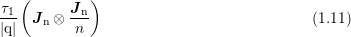 in
(1.7), and to neglect the contribution of velocity to the carrier energy, thus
in
(1.7), and to neglect the contribution of velocity to the carrier energy, thus
 This
leads to a parabolic system of equations and is a very common approximation in today’s device
simulators [30]. The two assumptions (1.11) and (1.12) can also be justified from a mathematical
point of view by a scaling argument for vanishing Knudsen number [84], which in addition shows
that the time derivatives in the flux equations vanish. This leads to the energy transport
model
This
leads to a parabolic system of equations and is a very common approximation in today’s device
simulators [30]. The two assumptions (1.11) and (1.12) can also be justified from a mathematical
point of view by a scaling argument for vanishing Knudsen number [84], which in addition shows
that the time derivatives in the flux equations vanish. This leads to the energy transport
model
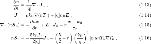 where (1.10) has been used. As the model consists of two conservation equations and two
constitutive equations, the name is slightly misleading.
where (1.10) has been used. As the model consists of two conservation equations and two
constitutive equations, the name is slightly misleading.
The closure based on Fourier’s law can be improved by taking the third moment of the BTE
into account [63]. A closure condition for the fourth-order tensor is obtained by assuming a
heated Maxwellian distribution, leading to
 instead of (1.16). This improved model based on four moments of the BTE is referred to as the
four moments energy transport model. A comparison of (1.16) and (1.17) reveals an inconsistency
of the energy transport model based on three moments, because the scalar prefactors in (1.16) are
given by
instead of (1.16). This improved model based on four moments of the BTE is referred to as the
four moments energy transport model. A comparison of (1.16) and (1.17) reveals an inconsistency
of the energy transport model based on three moments, because the scalar prefactors in (1.16) are
given by  and
and  , which means that the heat flux can be adjusted independently
[30].
, which means that the heat flux can be adjusted independently
[30].
1.1.4 The Six-Moments Model
With the drift-diffusion model based on two moments of the BTE, the hydrodynamic model based
on three moments and the energy transport model in modified form based on four moments of the
BTE, it is tempting to construct more accurate models based on higher moments. However, the
selection of suitable closure conditions becomes increasingly difficult. A model loosely based on
six moments of the BTE has been proposed by Sonoda et al. [98]. A rigorous derivation of a
model based on six moments has been carried out by Grasser et al. [29] in the diffusion limit of
vanishing Knudson number:
![∂n-= 1-∇ ⋅J , (1.18)
∂t |q| n
J = μk ∇ (nT )+ |q|nμE , (1.19)
n B n
∇ ⋅(nSn ) = − ∂nw-+ E ⋅J n − n w-−-w0-, (1.20)
∂t τ2
μS 5kBTn μS 5( kB )2
nSn = − ---------Jn − ----- --- |q|μnTn∇Tn , (1.21)
μ 2|q| μ 2 q
∇ ⋅ (nK ) = − 15-k2∂(nTn-Θn) − 2|q|E ⋅S − 15n TnΘn-−-T2L-, (1.22)
n 4 B ∂t n 4 τ4
35k3 μ [ |q| ]
nKn = ---B--kμn ∇ (nM6 )+ ---EnTn Θn . (1.23)
4 |q|μn kB](diss-et152x.png) The
additional unknown variables are the second order temperature
The
additional unknown variables are the second order temperature  and the kurtosis flux
  .
The parameter
.
The parameter  can be related to a mobility for kurtosis and
  is a macroscopic relaxation
time for the fourth moment of the scattering operator. A closure condition for the sixth moment
is a macroscopic relaxation
time for the fourth moment of the scattering operator. A closure condition for the sixth moment
 is obtained via the empirical relation
![(Θ )c
M6 = T3n --n , c ∈ [0,3] . (1.24)
Tn](diss-et158x.png) A
value of
A
value of  for the parameter
  proved to provide highest accuracy when compared to Monte
Carlo results and further shows higher numerical stability than other choices. Particularly, the
Newton procedure for the choice
proved to provide highest accuracy when compared to Monte
Carlo results and further shows higher numerical stability than other choices. Particularly, the
Newton procedure for the choice  has been reported to result in failure of convergence in
most cases.
has been reported to result in failure of convergence in
most cases.
1.1.5 The Monte Carlo Method
The macroscopic transport models presented so far are specified by a system of partial differential
equations which approximate certain features of the BTE, for which suitable deterministic
numerical solutions are sought. A stochastic approach for the solution of the full BTE
is the Monte Carlo method, where the dynamics are simulated at the particle level
[52, 47] and which was already used in the 1960s for semiconductor device simulations
(e.g. [61]). The free streaming operator of the BTE is obtained from Newton’s laws of
motion
 while
the scattering operator models instantaneous changes of the momentum of each particle in the
device. Denote with
while
the scattering operator models instantaneous changes of the momentum of each particle in the
device. Denote with  the conditional probability of finding a particle at
location
the conditional probability of finding a particle at
location  with wave vector
  at time
  given that the particle was at location
  with wave
vector
with wave
vector  at time
  . Since not only the distribution function
  , but also
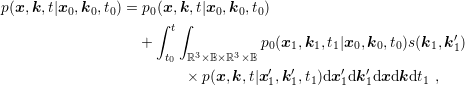
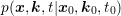 satisfies the BTE, a formal integration of the BTE after merging the
gradients with respect to
satisfies the BTE, a formal integration of the BTE after merging the
gradients with respect to  and
and  into a joint gradient for the variable
  yields
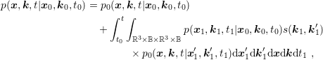 | (1.26) |
where  denotes the Brillouin zone and
 is the
conditional probability of finding a particle in state
is the
conditional probability of finding a particle in state  at time
  given that the particle was
located at
given that the particle was
located at  with wave vector
  at time
  without being scattered.
  and
and  are
shorthand notations for the location of the particle at a given instance in time for a given initial
position. Eq. (1.26) is an integral equation for
are
shorthand notations for the location of the particle at a given instance in time for a given initial
position. Eq. (1.26) is an integral equation for  , and the conjugate
form
, and the conjugate
form
 | (1.28) |
is the basis for the usual Monte Carlo algorithm.
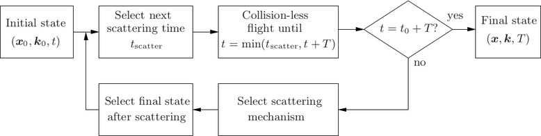
The Monte Carlo procedure uses a large sample of particles and simulates their dynamic
behavior based on the integral formulation (1.28). To this end, the time intervals between the
scattering events of each particle are chosen randomly based on the scattering operator, and
particles propagate in collision-less flight according to (1.25) between scattering events.
Macroscopic quantities such as average carrier energies are computed by suitable averages over
the particle ensemble. In order to keep stochastic fluctuations reasonably small, a large
number of particles is required, where the accuracy is asymptotically proportional
to the square-root of the execution time unless special enhancement techniques for
selected target quantities are applied [52]. While the Monte Carlo method provides a
very high accuracy due to the simulation of particle kinetics and high flexibility with
respect to the inclusion of additional physical details, it is computationally extremely
expensive.
1.2 Requirements of Modern TCAD
The various transport models and solution approaches to the BTE discussed in the previous
section represent only a selection of the most popular methods for the simulation of charge
transport in semiconductors. Regarding their accuracy and computational cost, these models
typically range from the computationally cheap drift-diffusion model, which fails to reflect physics
properly in the deca-nanometer regime, to the accurate Monte Carlo method, which has the
drawback of extremely high computational costs. In the following, a discussion of the
requirements of a state-of-the-art semiconductor device simulator is given. The individual
requirements slightly overlap, but they should aid the reader in judging the importance of the
proposed extensions of the deterministic Boltzmann solution method given in the remainder of
this thesis.
1.2.1 Accuracy
The need for a better reflection of the underlying physical processes compared to the
drift-diffusion model has lead to the development of higher-order transport models such
as the hydrodynamic model. As device dimensions decrease, ballistic effects become
significant, which cannot be captured in the diffusion-limited regime of higher-order
transport models [51, 30]. As a consequence, it is desireable to have numerical methods
which are computationally less expensive than the Monte Carlo method, but are able
to resolve ballistic transport effects. Even though not covered by the semiclassical
approach, quantum effects become increasingly important and should be reflected in the
model.
1.2.2 Charge Conservation
Kirchhoff’s current law states the conservation of charge. Consequently, charge conservation has
to be ensured during the simulation of a single semiconductor device as well. The use of the box
integration scheme for the drift-diffusion model guarantees charge conservation at the algebraic
level. Similarly, charge conservation is provided for other moment-based methods. Moreover, the
particle approach of the Monte Carlo method allows for charge conservation without difficulties.
As a consequence, new simulation approaches need to ensure charge conservation in order to be
competitive with existing methods.
1.2.3 Self-Consistency
The electrostatic potential and the space charge are linked by the Poisson equation, which is a
direct implication of Gauss’ Law. Since it is in general neither possible to explicitly
express the potential as a function of the carrier densities, nor to express the carrier
densities as an explicit function of the electrostatic potential only, any transport model
used for charge transport is required to be solved self-consistently with the Poisson
equation.
1.2.4 Resolution of Complicated Domains
With the on-going miniaturization of semiconductor devices, inherent small variations in
the fabrication process become significant with respect to the characteristic device
lengths. Consequently, device geometries are no longer simple compositions of geometric
primitives, but should be taken from topography simulations. Therein, complicated device
geometries show up in a natural way, particularly for fully three-dimensional device
layouts.
1.2.5 Computational Feasibility
The incredible pace of semiconductor device technology requires that simulation results are
available within a short time frame. In particular, simulation times in the range of weeks or even
months are clearly not acceptable, because during that time technology has progressed and
simulation results may be deprecated already before they are available. This is the main reason
why Monte Carlo methods are – despite their high accuracy – not commonly used for every-day
TCAD purposes.
1.2.6 Extendibility
As devices are scaled down, formerly negligible physical effects become relevant and need to be
considered in the simulation. Thus, it is desirable to use numerical methods which allow for such
an inclusion without a large redesign of the whole simulator. For instance, boundary element
methods based on the knowledge of the Green’s function of the underlying partial differential
equations become invalid and eventually infeasible as soon as details such as e.g. space-dependent
diffusion coefficients are demanded.
1.3 Outline
The remainder of this thesis focuses on a rather new approach based on a spherical harmonics
expansion of the distribution function. The method is expected to yield the accuracy of Monte
Carlo methods without the inherent disadvantages of stochastic models. Other approaches for the
deterministic numerical solution of the BTE have been proposed, but they are considered to be
limited to at most two-dimensional device geometries either because the full momentum space
needs to be discretized [19, 14], or because the discretization method leads to nonlocal couplings
resulting in huge memory requirements for the resulting linear system of equations
[72].
In Chap. 2 an introduction to the SHE method is given and the state-of-the-art for the
method is presented, excluding the extensions proposed in this work. The chapter closes
with a discussion of the compatibility of the SHE method with respect to modern
TCAD.
Chap. 3 details the underlying physical processes and their consideration within the SHE
method. A method for the inclusion of carrier-carrier scattering is proposed at the end of the
chapter.
The mathematical structure of the SHE equations is investigated in detail in Chap. 4. A
sparse coupling property of the SHE equations is shown for spherical energy bands.
These coupling investigations then lead to a system matrix compression scheme, which
allows for a memory efficient representation of the system matrix at high expansion
orders.
Chap. 5 presents the extension of the SHE method to unstructured grids. All the required
implementation details for the construction of suitable meshes are given.
In order to obtain the accuracy of higher-order expansions at lower computational effort,
adaptive variable-order expansions are proposed and evaluated in Chap. 6. The possible savings
mostly stem from the fact that on the one hand the distribution function is still close to
equilibrium in inactive device regions, and on the other hand from the asymptotically exponential
decay of the distribution function with respect to kinetic energy, hence lower resolution at higher
energies is sufficient.
Recent developments in computing architecture are addressed in Chap. 7, where a parallel
scheme for the convergence enhancement of the iterative solvers by means of preconditioners is
suggested. It enables the full utilization of multi-core central processing units as well
as the efficient use with massively parallel architectures such as graphics processing
units.
The suggestions from Chaps. 4 to 7 are combined for the simulation of a MOSFET and a
FinFET in Chap. 8. It is demonstrated that the proposed techniques blend well with each other
and render the SHE method very attractive for modern TCAD.
An outlook to further possible improvements of the SHE method is presented in Chap. 9. A
conclusion finally closes this thesis.
 to
to  .
.