Chapter 7
Parallelization
The paradigm shift from single- to multi- and many-core computing architectures places
additional emphasis on the development of parallel algorithms. In particular, the use of graphics
processing units (GPUs) for general purpose computations poses a considerable challenge due to
the high number of threads executed in parallel. Already the implementation of standard
algorithms like dense matrix-matrix multiplications requires a considerable amount
of sophistication in order to utilize the vast computing resources of GPUs efficiently
[70].
In the context of the discretized SHE equations (5.9) and (5.16), the assembly can be carried
out in parallel for each box  and each adjoint box
  , provided a suitable storage
scheme for the sparse system matrix is chosen. Similarly, the elimination of odd-order unknowns
from the system matrix can be achieved in parallel, since the procedure can be carried out
separately for each row associated with a box
, provided a suitable storage
scheme for the sparse system matrix is chosen. Similarly, the elimination of odd-order unknowns
from the system matrix can be achieved in parallel, since the procedure can be carried out
separately for each row associated with a box  of the system matrix. The iterative solvers
essentially rely on sparse matrix-vector products, inner products and vector updates,
which can also be run in parallel employing parallel reduction schemes. However, the
additional need for preconditioners is a hindrance for a full parallelization, because the
design of good parallel preconditioners is very challenging and typically problem-specific
[104].
of the system matrix. The iterative solvers
essentially rely on sparse matrix-vector products, inner products and vector updates,
which can also be run in parallel employing parallel reduction schemes. However, the
additional need for preconditioners is a hindrance for a full parallelization, because the
design of good parallel preconditioners is very challenging and typically problem-specific
[104].
In this chapter a parallel preconditioning scheme for the SHE equations is proposed and
evaluated. The physical principles on which the preconditioner is based are discussed in Sec. 7.1
and additional numerical improvements for the system matrix are given in Sec. 7.2.
The preconditioner scheme is then proposed in Sec. 7.3 and evaluated for a simple
 -diode in Sec. 7.4. Even though parallel preconditioners suitable for GPUs
have already been implemented recently, cf. e.g. [33, 40], their black-box nature does
not make full use of all available information. The preconditioner scheme presented
in the following incorporates these additional information into otherwise black-box
preconditioners.
-diode in Sec. 7.4. Even though parallel preconditioners suitable for GPUs
have already been implemented recently, cf. e.g. [33, 40], their black-box nature does
not make full use of all available information. The preconditioner scheme presented
in the following incorporates these additional information into otherwise black-box
preconditioners.
The scheme is derived for a given electrostatic potential, as it is for instance the case with a
Gummel iteration, cf. Sec. 2.4. A block-preconditioner for the Newton scheme is obtained by
concatenation of a preconditioner for the Poisson equation, the SHE preconditioner presented in
the following, and a preconditioner for the continuity equation for the other carrier
type.
7.1 Energy Couplings Revisited
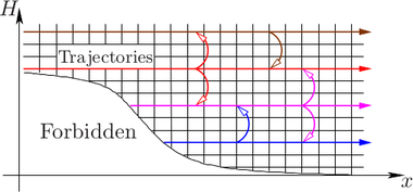
As discussed in Chap. 3, carriers within the device can change their total energy only by inelastic
scattering events, thus the scattering operator  is responsible for coupling different
energy levels. However, if only elastic scattering processes are considered, the total energy of the
particles remains unchanged and the different energy levels do not couple, cf. Fig. 7.1. Therefore,
in a SHE simulation using only elastic scattering and
is responsible for coupling different
energy levels. However, if only elastic scattering processes are considered, the total energy of the
particles remains unchanged and the different energy levels do not couple, cf. Fig. 7.1. Therefore,
in a SHE simulation using only elastic scattering and  different energy levels, the resulting
system of linear equations is consequently decoupled into
different energy levels, the resulting
system of linear equations is consequently decoupled into  independent problems. Such a
decomposition has been observed already in early publications on SHE [21, 105] in a slightly
different setting: If the grid spacing with respect to energy is a fraction of the optical
phonon energy
independent problems. Such a
decomposition has been observed already in early publications on SHE [21, 105] in a slightly
different setting: If the grid spacing with respect to energy is a fraction of the optical
phonon energy  , say
, say  with integer
  , then the system decomposes into
 decoupled systems of equations. This observation, however, is of rather limited
relevance in practice, since different phonon energies
decoupled systems of equations. This observation, however, is of rather limited
relevance in practice, since different phonon energies  for inelastic scattering may be
employed simultaneously, cf. Sec. 3.3, hence the system no longer decouples into a
reasonably large number of independent systems in order to scale well to a higher number of
cores.
for inelastic scattering may be
employed simultaneously, cf. Sec. 3.3, hence the system no longer decouples into a
reasonably large number of independent systems in order to scale well to a higher number of
cores.
It is assumed throughout the following investigations that all unknowns of the discrete linear
system of equations referring to a certain energy  are enumerated consecutively. A simple
interpretation of the system matrix structure is possible if first all unknowns associated with the
lowest energy
are enumerated consecutively. A simple
interpretation of the system matrix structure is possible if first all unknowns associated with the
lowest energy  are enumerated, then all unknowns with energy
  and so forth. The
unknowns for a certain energy can be enumerated arbitrarily, even though an enumeration
such as in Sec. 6.1 is of advantage for easing the understanding of the system matrix
structure.
and so forth. The
unknowns for a certain energy can be enumerated arbitrarily, even though an enumeration
such as in Sec. 6.1 is of advantage for easing the understanding of the system matrix
structure.
The scattering of carriers is a random process in the sense that the time between two collisions
of a particle are random. Equivalently, the mean free flight denotes the average distance a carrier
travels before it scatters. As devices are scaled down, the average number of scattering
events of a carrier while moving through the device decreases. On the algebraic level of
the system matrix, a down-scaling of the device leads to a weaker coupling between
different energy levels. This can be reasoned as follows: Consider a one-dimensional device
using spherical energy bands, consisting of two boxes  and
and  with adjoint box
 . Now, consider the discretization (5.9) and (5.16). In the following, only the
proportionality with respect to the box interface area and the box volume are of interest.
Consequently,
. Now, consider the discretization (5.9) and (5.16). In the following, only the
proportionality with respect to the box interface area and the box volume are of interest.
Consequently,  is written for a term that carries a dependence on the interface area
 , and
, and  is written for a term that depends on the box volumes
  or
or  .
Since only the asymptotic behavior is of interest, the signs are always taken positive.
The discrete system matrix can then be written according to (5.9) and (5.16) in the
form
.
Since only the asymptotic behavior is of interest, the signs are always taken positive.
The discrete system matrix can then be written according to (5.9) and (5.16) in the
form
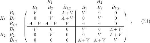 where the three rows and columns in each energy block refer to the assembly of the boxes
  ,
,
 and
and  . An elimination of the odd-order unknowns, i.e. rows and columns three and six,
leads to
. An elimination of the odd-order unknowns, i.e. rows and columns three and six,
leads to
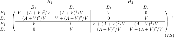 where again all signs were taken positive for simplicity, since only the asymptotics are of interest.
For characteristic box diameter
where again all signs were taken positive for simplicity, since only the asymptotics are of interest.
For characteristic box diameter  in an
in an  -dimensional real space there holds
  and
and
 , thus the matrix structure when keeping only the lowest powers of
  for each entry is
asymptotically given by
for each entry is
asymptotically given by
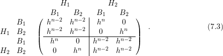 Hence, the off-diagonal blocks coupling different energies become negligible as devices are shrunk.
The same asymptotics hold true for an arbitrary number of boxes and energy levels, hence the
physical principle of reduced scattering of carriers while travelling through the device is well
reflected on the discrete level.
Hence, the off-diagonal blocks coupling different energies become negligible as devices are shrunk.
The same asymptotics hold true for an arbitrary number of boxes and energy levels, hence the
physical principle of reduced scattering of carriers while travelling through the device is well
reflected on the discrete level.
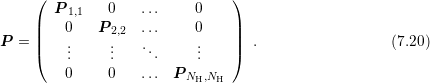
7.2 Symmetrization of the System Matrix
With the enumeration of unknowns as suggested in the previous section and using only a single
inelastic phonon energy  , the structure of the system matrix consists of three block-diagonals.
The location of the off-diagonal blocks depends on the spacing of the discrete energies
with respect to
, the structure of the system matrix consists of three block-diagonals.
The location of the off-diagonal blocks depends on the spacing of the discrete energies
with respect to  . If the energy spacing equals
  , the matrix is block-tridiagonal,
cf. Fig. 7.2.
, the matrix is block-tridiagonal,
cf. Fig. 7.2.
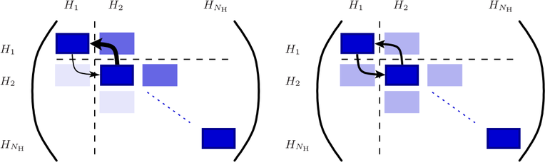
Figure 7.2: Structure of the system matrix for total energy levels 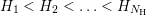 with an energy grid spacing equal to the inelastic energy
  before (left) and after (right)
symmetrization. Unknowns at the same total energy
before (left) and after (right)
symmetrization. Unknowns at the same total energy  are enumerated consecutively,
inducing a block-structure of the system matrix. For simplicity, scattering is depicted
between energy levels
are enumerated consecutively,
inducing a block-structure of the system matrix. For simplicity, scattering is depicted
between energy levels  and
and  only, using arrows with thickness proportional to the
magnitude of the entries.
only, using arrows with thickness proportional to the
magnitude of the entries.
The asymptotic exponential decay of the distribution function with energy induces a
considerable asymmetry of the system matrix when inelastic scattering is considered. This
asymmetry, however, is required in order to ensure a Maxwell distribution in equilibrium.
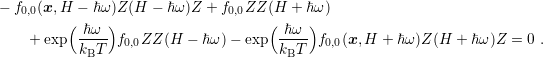
Consider the scattering rate (3.25) and the SHE equations for the scattering operator only. The
resulting equations for the zeroth-order expansion coefficients using spherical energy bands
read
 | (7.4) |
where the symmetric scattering rate  has been cancelled already. The first two terms refer to
scattering from lower to higher energy, and the last two terms to scattering from higher energy to
lower energy. Substitution of the relation
has been cancelled already. The first two terms refer to
scattering from lower to higher energy, and the last two terms to scattering from higher energy to
lower energy. Substitution of the relation
 and
division by
and
division by  leads to
 | (7.6) |
It can readily be seen that a Maxwell distribution  fulfills the
equation. For the system matrix one consequently finds that the off-diagonal block coupling to
higher energy is by a factor of
fulfills the
equation. For the system matrix one consequently finds that the off-diagonal block coupling to
higher energy is by a factor of  larger than the block coupling to lower energy.
For phonon energies of about
larger than the block coupling to lower energy.
For phonon energies of about  meV the factor is
  , while for phonon
energies
, while for phonon
energies  meV the factor becomes
  . The induced asymmetry of the system
matrix is in particular a concern for the convergence of iterative solvers if the off-diagonal block
coupling to higher energies dominates the diagonal block, which is typically the case for devices in
the micrometer regime.
. The induced asymmetry of the system
matrix is in particular a concern for the convergence of iterative solvers if the off-diagonal block
coupling to higher energies dominates the diagonal block, which is typically the case for devices in
the micrometer regime.
The asymmetry can be substantially reduced in two ways. The first possibility is to expand
the distribution function as
 where
where  is a reasonable estimate for
  . A first guess for the first iteration of a
self-consistent iteration is a Maxwell distribution,
. A first guess for the first iteration of a
self-consistent iteration is a Maxwell distribution,
 which can be refined in subsequent iterations with the shape of the computed distribution
function from the last iterate. A disadvantage of the expansion (7.7) is that the SHE
equations need to be slightly adjusted and thus depend on the scaling
which can be refined in subsequent iterations with the shape of the computed distribution
function from the last iterate. A disadvantage of the expansion (7.7) is that the SHE
equations need to be slightly adjusted and thus depend on the scaling  . However,
the discrete representations (5.4) and (5.5) approximate the expansion coefficients
and hence the distribution function as piecewise constant over the boxes in
. However,
the discrete representations (5.4) and (5.5) approximate the expansion coefficients
and hence the distribution function as piecewise constant over the boxes in  and
and
 . While this is a crude approximation for the exponentially decaying expansion
coefficients
. While this is a crude approximation for the exponentially decaying expansion
coefficients  of the exponentially decaying distribution function
  using the
standard expansion
using the
standard expansion  , an expansion of the form (7.7) leads to much smaller
variations of the expansion coefficients
, an expansion of the form (7.7) leads to much smaller
variations of the expansion coefficients  . Consequently, the exponential decay is
basically covered by
. Consequently, the exponential decay is
basically covered by  , and a piecewise constant approximation of
  is more
appropriate.
is more
appropriate.
The second way of reducing asymmetry is based on modifications of the linear system.
Denoting again with  a reasonable estimate for
  , the system of linear equations
with eliminated odd expansion orders
, the system of linear equations
with eliminated odd expansion orders
 can
be rewritten as
can
be rewritten as
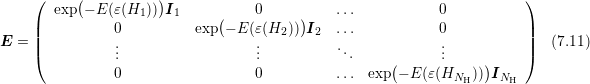
 where
where  is given in block structure as
 with
with
 referring to an identity matrix with dimensions given by the unknowns at energy level
  .
Introducing
.
Introducing  and
and  , one arrives at
 Since
Since  is a diagonal matrix, the costs of computing
  and
and  are comparable to a
matrix-vector product and thus negligible. The benefit of this rescaling is that the
unknowns computed in vector
are comparable to a
matrix-vector product and thus negligible. The benefit of this rescaling is that the
unknowns computed in vector  are roughly of the same magnitude and that the
off-diagonal coupling entries in each row of
are roughly of the same magnitude and that the
off-diagonal coupling entries in each row of  are essentially identical. It should be noted
that the rescaling on the discrete level is actually a special case of an expansion of the
form (7.7), where
are essentially identical. It should be noted
that the rescaling on the discrete level is actually a special case of an expansion of the
form (7.7), where  is taken constant in each box of the simulation domain in
 -space.
A second look at the rescaled system matrix  shows that norms of the columns
are now exponentially decreasing with energy, while the column norms of
shows that norms of the columns
are now exponentially decreasing with energy, while the column norms of  are
of about the same order of magnitude. Hence, the rescaling with
are
of about the same order of magnitude. Hence, the rescaling with  has shifted the
exponential decay of the entries in
has shifted the
exponential decay of the entries in  to the columns of the system matrix. However,
due to the block structure of the system matrix, a normalization of the row-norms by
left-multiplication of the linear system with a diagonal matrix
to the columns of the system matrix. However,
due to the block structure of the system matrix, a normalization of the row-norms by
left-multiplication of the linear system with a diagonal matrix  also rescales the column-norms
suitably:
also rescales the column-norms
suitably:
 where
where
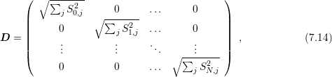 with
with
 denoting the number of rows in
  . Again, the application of
  is computationally cheap
and leads with
is computationally cheap
and leads with  and
and  to the linear system
 It is
worthwhile to note that the diagonal entries of
It is
worthwhile to note that the diagonal entries of  are essentially proportional to
 and thus represent the MEDS factors from Sec. 2.3. In addition, also the
exponential decay of values in
and thus represent the MEDS factors from Sec. 2.3. In addition, also the
exponential decay of values in  due to Maxwell distributions induced by suitable
boundary conditions is automatically rescaled to values in about the same order of
magnitude.
due to Maxwell distributions induced by suitable
boundary conditions is automatically rescaled to values in about the same order of
magnitude.
7.3 A Parallel Preconditioning Scheme
Due to the large number of unknowns for the discretized SHE equations, the solution of the
resulting systems of linear equations is typically achieved by iterative methods. The rate of
convergence of these methods can be substantially improved by the use of preconditioners. As
already observed by Jungemann et al. [53], good preconditioners are actually required in most
cases to obtain convergence of iterative solvers for the SHE equations. One of the most commonly
employed preconditioners is the incomplete LU factorization (ILU), which has been used in recent
works on the SHE method [53, 42]. For this reason, a short description of ILU is given in the
following.
ILU relies on an approximate factorization of the sparse system matrix  into
into
 , where
  is a sparse lower triangular matrix, and
  is a sparse upper
triangular matrix. During the iterative solver run, the current residual
is a sparse upper
triangular matrix. During the iterative solver run, the current residual  is then updated
by
is then updated
by
 in
order to formally solve the system
in
order to formally solve the system
 rather than
  . If
. If  , i.e. the factorization is exact, the solution is obtained in
one step. Conversely, if
, i.e. the factorization is exact, the solution is obtained in
one step. Conversely, if  is the identity matrix, the linear system is solved as if no
preconditioner were employed.
is the identity matrix, the linear system is solved as if no
preconditioner were employed.
The inverse of  is never computed explicitly. Instead, a forward substitution
  followed by a backward substitution
  is carried out. Since these substitutions are serial
operations, the application of the preconditioner to the residual is identified as a bottleneck for
parallelism.
is carried out. Since these substitutions are serial
operations, the application of the preconditioner to the residual is identified as a bottleneck for
parallelism.
In light of the discussion of the block structure of the system matrix  for SHE, consider a
block-diagonal matrix
for SHE, consider a
block-diagonal matrix
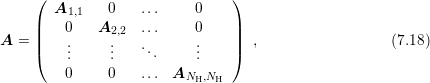 where the
  square blocks of
  can have arbitrary size. Then, the solution of the
system
can have arbitrary size. Then, the solution of the
system
 can
be obtained by solving each of the systems
can
be obtained by solving each of the systems  for the respective subvectors
  and
and
 separately. Denoting with
  the preconditioner for
  , the preconditioner for the full
system
, the preconditioner for the full
system  is consequently also given in block diagonal form
 Since
the purpose of a preconditioner is to approximate the inverse of the system matrix, the
block-diagonal preconditioner
Since
the purpose of a preconditioner is to approximate the inverse of the system matrix, the
block-diagonal preconditioner  will provide a good approximation to the inverse of
  even if
  is not strictly block diagonal, but has small entries in off-diagonal blocks.
However, this is exactly the case for the system matrix resulting from the SHE equations
discussed in Sec. 7.1. Summing up, the proposed preconditioning scheme reads as
follows:
is not strictly block diagonal, but has small entries in off-diagonal blocks.
However, this is exactly the case for the system matrix resulting from the SHE equations
discussed in Sec. 7.1. Summing up, the proposed preconditioning scheme reads as
follows:
A physical interpretation of the proposed preconditioner is as follows: Consider the
discretization of the SHE equations without inelastic scattering mechanisms. In this case the
system matrix  after row-normalization is block-diagonal if enumerating the
unknowns as suggested in Sec. 7.1. A preconditioner for
after row-normalization is block-diagonal if enumerating the
unknowns as suggested in Sec. 7.1. A preconditioner for  is given by a block
preconditioner
is given by a block
preconditioner  of the form (7.20). Since
  is an approximation to the SHE
equations with inelastic scattering given by
is an approximation to the SHE
equations with inelastic scattering given by  , for a preconditioner
  for
for  there
holds
there
holds
 The use of the block diagonals of
  rather than the matrix
  for the setup
of the preconditioner
for the setup
of the preconditioner  is of advantage because it avoids the setup of the matrix
 .
.
It should be noted that the use of block preconditioners of the form (7.20) for the
parallelization of ILU preconditioners is not new [88]. However, without additional information
about the system matrix, the block sizes are usually chosen uniformly and may not be aligned to
the block sizes induced by the SHE equations. Consequently, the application of block-diagonal
preconditioners to the SHE equations in a black-box manner will show lower computational
efficiency.
The proposed scheme in Algorithm 5 allows for the use of arbitrary preconditioners for each of
the blocks  . Consequently, a preconditioner scheme is proposed rather than a
single preconditioner, enabling the use of established serial preconditioners in a parallel
setting. Since the number of energies
. Consequently, a preconditioner scheme is proposed rather than a
single preconditioner, enabling the use of established serial preconditioners in a parallel
setting. Since the number of energies  is in typical situations chosen to be at least
 , the proposed scheme provides a sufficiently high degree of parallelism even for
multi-CPU clusters. The situation is slightly different for GPUs, where typically one work
group
is used for the preconditioner at total energy
, the proposed scheme provides a sufficiently high degree of parallelism even for
multi-CPU clusters. The situation is slightly different for GPUs, where typically one work
group
is used for the preconditioner at total energy  . Due to the massively parallel architecture of
GPUs, an even higher degree of parallelism is desired in order to scale the SHE method well to
multi-GPU environments. In such case, parallel preconditioner for each block
. Due to the massively parallel architecture of
GPUs, an even higher degree of parallelism is desired in order to scale the SHE method well to
multi-GPU environments. In such case, parallel preconditioner for each block  should be
employed.
should be
employed.
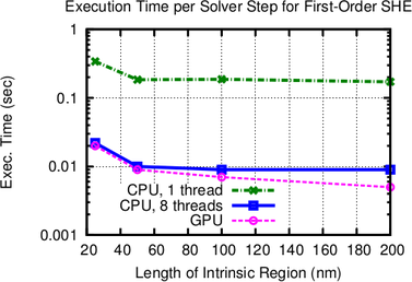
7.4 Results
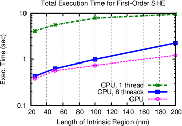
Execution times of the iterative BiCGStab [102] solver are compared for a single CPU core using
an incomplete LU factorization with threshold (ILUT) for the full system matrix, and for the
proposed parallel scheme using multiple CPU cores of a quad-core Intel Core i7 960 CPU
with eight logical cores. In addition, comparisons for a NVIDIA Geforce GTX 580
GPU are found in Figs. 7.3. The parallelization on the CPU is achieved using the
Boost.Thread library [6], and the same development time was allotted for developing the
OpenCL [57] kernel for ViennaCL [111] on the GPU. This allows for a comparison of
the results not only in terms of execution speed, but also in terms of productivity
[7].
As can be seen in Figs. 7.3, the performance increase for each linear solver step is more than
one order of magnitude compared to the single-core implementation. This super-linear scaling
with respect to the number of cores on the CPU is due to the better caching possibilities obtained
by the higher data locality within the block-preconditioner.
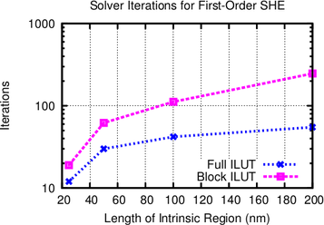
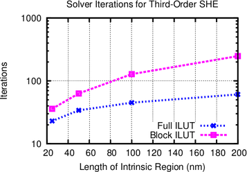
The required number of iterations using the block-preconditioner decreases with the device
size. For an intrinsic region of  nm length, the number of iterations is only twice than that of
an ILUT preconditioner for the full system. At an intrinsic region of
nm length, the number of iterations is only twice than that of
an ILUT preconditioner for the full system. At an intrinsic region of  nm, four times the
number of iterations are required. This is a very small price to pay for the excellent parallelization
possibilities.
nm, four times the
number of iterations are required. This is a very small price to pay for the excellent parallelization
possibilities.
Overall, the multi-core implementation is on the test machine by a factor of three to ten faster
than the single core-implementation even though a slightly larger number of solver iterations is
required. It is reasonable to expect even higher performance gains on multi-socket machines
equipped with a higher number of CPU cores. The purely GPU-based solver with hundreds of
simultaneous lightweight threads is by up to one order of magnitude faster than the single-core
CPU implementation, where it has to be noted that a single GPU thread provides less processing
power than a CPU thread.
The comparison in Fig. 7.3 further shows that the SHE order does not have a notable
influence on the block-preconditioner efficiency compared to the full preconditioner. The slightly
larger number of solver iterations for third-order expansions is due to the higher number of
unknowns in the linear system. The performance gain is almost uniform over the length of the
intrinsic region and slightly favors shorter devices, thus making the scheme an ideal candidate for
current and future scaled-down devices.
 .
. 


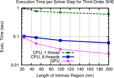
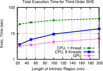
 diodes with different lengths of the intrinsic region. As expected from physical arguments,
the parallel preconditioner performs the better the smaller the length of the intrinsic
region becomes. The GPU version performs particularly well for the computationally
more challenging third-order SHE. A reduction of total execution times compared to a
single-threaded implementation by one order of magnitude is obtained.
diodes with different lengths of the intrinsic region. As expected from physical arguments,
the parallel preconditioner performs the better the smaller the length of the intrinsic
region becomes. The GPU version performs particularly well for the computationally
more challenging third-order SHE. A reduction of total execution times compared to a
single-threaded implementation by one order of magnitude is obtained.