| | |
Having carefully prepared the foundations which present the scenery for the geometrical considerations at hand, it is time to turn to geometric entities. It is again prudent to present a very simple case first, which allows to build higher structures upon.
Definition 45 (Curve) A smooth map of an interval  to a differentiable manifold
  (Definition 37) is called a curve:

Two curves are not identical, in the strictest of senses, if their images coincide, while their parametrization differ.
Using a curve, every number  is mapped to a point of
  , which may be used as input for
the charts of the manifold (Definition 35), thereby effectively creating the new mapping:
, which may be used as input for
the charts of the manifold (Definition 35), thereby effectively creating the new mapping:
This pullback (Definition 44) by the charts also results in coordinate representations for the involved points. While the properties of a considered curve do not depend on the choice of a particular coordinate system, the mere existence of the mapping allows to explain the concept of a differentiable curve.
Definition 46 (Differentiable curve) A curve  is considered to be differentiable, if the
functions describing its coordinate representations
is considered to be differentiable, if the
functions describing its coordinate representations  as defined by Equation 4.64 are
differentiable functions.
as defined by Equation 4.64 are
differentiable functions.
Having defined differentiable curves, it is only fitting to recall basic mathematics and how tangents to graphs of simple functions may be linked to differentials, and extend the concept by applying similar reasoning in this setting.
The differentiation is with respect to a single parameter and touches the coordinate expressions according to Equations 4.64.
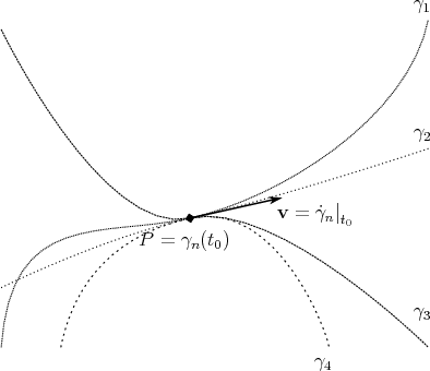
Figure 4.3 illustrates that Definition 47 can be met by several, in fact infinitely many, curves. However, recalling Definition 9 it is possible to extract essential parts of information which leads to the following definition introducing a key geometric entity.
Definition 48 (Tangent vector space) Considering the set of all curves passing through a point
 , the identity of the first derivatives defines a set of equivalence classes (Definition 9):
![˙γ = [γ ] (4 .67)](whole304x.png)
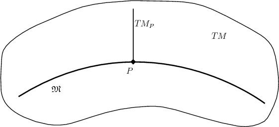
 define a space
  , which carries the structure of a vector
space (Definition 16) and tangent to
, which carries the structure of a vector
space (Definition 16) and tangent to  at the point
  . The dimensions of the manifold
  and
and
 are identical

The vectors now available after Definition 48 alone do not suffice to easily develop complex models of physical processes. A method of evaluation, a measurement, of the vectors is also required, which motivates the next definition.
Definition 49 (Dual vector space) Given a vector space  , its dual space
  is comprised by the
linear functionals
is comprised by the
linear functionals

The dual space  also carries the structure of a vector space (Definition 16), its elements are called
co-vectors or one-forms. In particular it is possible to define a non-degenerate bilinearform, called the
scalar product.
also carries the structure of a vector space (Definition 16), its elements are called
co-vectors or one-forms. In particular it is possible to define a non-degenerate bilinearform, called the
scalar product.

 may only occur, if either

In finite dimensions, the dimensions of two dual vector spaces are equal.

Definition 50 (Cotangent vector space) The dual space of the tangent vector space is called
the cotangent vector space  .
.
In the case of infinite-dimensional vector spaces such as the spaces of functions, a slight modification is required. When dealing with infinite dimensions, the topological dual space is defined by demanding the linear functionals to be continuous. In finite dimension this demand is not required explicitly, since all linear functionals are inherently continuous.
Before proceeding further it is necessary to clarify another piece of terminology connecting Definition 40 and Definition 16.
Definition 51 (Vector bundle) A fiber bundle (Definition 40), where the fibers  carry the
structure of a vector space (Definition 16), is called a vector bundle.
carry the
structure of a vector space (Definition 16), is called a vector bundle.
Definition 52 ((Co)Tangent bundle) The (co)tangent spaces  (
( ) (Definition 48) are
parametrized on the points
) (Definition 48) are
parametrized on the points  . The disjoint union of all (co)tangent spaces
 . The manifold is the base space, while
the tangent spaces at each of the points
. The manifold is the base space, while
the tangent spaces at each of the points  are the attached fibers.
The structure of a (co)tangent bundle  (
( ) of a smooth manifold
  (Definition 37) is again
a smooth manifold.
(Definition 37) is again
a smooth manifold.
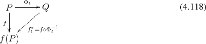
A particular mapping between the tangent and co-tangent bundle will be interesting in conjunction with Section 5.3 and is thus introduced here.
Definition 53 (Legendre map) The Legendre map is a mapping between the tangent and the
cotangent bundle (Definition 52) of a manifold  (Definition 37)

 (Definition 25)

 vectors from a fiber over
  it is related to a function


Similar to the introduction of the elements of the dual vector space, the 1-forms, it is possible to define more complex mappings not only from the vector space but also its dual to the field above which the vector space has been constructed.
In this context the original vectors and 1-forms appear as the special cases of  and
and  tensors
respectively. The collection of all tensors of type
tensors
respectively. The collection of all tensors of type  based on the vector space
  again has the
structure of a vector space and shall be denoted by
again has the
structure of a vector space and shall be denoted by  . The dimension of this vector space
is
. The dimension of this vector space
is

While the bases of the tangent and co-tangent vector spaces can be linked to the charts of the manifold
 , this is so far not available for the vector space of tensors. It is therefore desirable to
have a mapping available which, among other things, enables the determination of bases for
the tensors spaces of arbitrary dimension from the initial tangent and co-tangent spaces.
, this is so far not available for the vector space of tensors. It is therefore desirable to
have a mapping available which, among other things, enables the determination of bases for
the tensors spaces of arbitrary dimension from the initial tangent and co-tangent spaces.
Definition 55 (Tensor product) The non-commutative and associative mapping

is called a tensor product.
Tensors with their algebraic structures represent a very abstract and powerful concept with considerable
applicability.The notion of a tensor and its properties do not rely on the particular choice of its
representation. The properties do not specify, however, how a particular tensor is defined and how to
obtain its corresponding value for a given input. Coordinates with respect to a given choice of base  provide a means to address this problem.
The linear structure of tensors and using the tensor product (Definition 55) allows to express any tensor
 in the form of
 are the coordinates of the tensor
  in the base elements
  . Providing the full set of
tensor coordinates along with the base they refer to, completely specifies the tensor. This important fact
is quite commonly abused attributing special properties to the coordinates themselves and in fact
considering tensors and vectors alike as little more then a suitable collection of values as found, for
example, in matrix representations. While indispensable, a reduction to this primitive level of
abstraction belies the true structure of the entities at hand. A tendency of this reductionism has even
been compared to a mathematical disease [76]. Where this regression of abstraction may be tedious
from a theoretical setting, its severity only increases in the case that properties should be qualified from
the coordinates, when they are subjected to calculations of limited precision. It is therefore highly
desirable to retain as much abstract information as possible in both theoretical as well as practical
fields.
. Providing the full set of
tensor coordinates along with the base they refer to, completely specifies the tensor. This important fact
is quite commonly abused attributing special properties to the coordinates themselves and in fact
considering tensors and vectors alike as little more then a suitable collection of values as found, for
example, in matrix representations. While indispensable, a reduction to this primitive level of
abstraction belies the true structure of the entities at hand. A tendency of this reductionism has even
been compared to a mathematical disease [76]. Where this regression of abstraction may be tedious
from a theoretical setting, its severity only increases in the case that properties should be qualified from
the coordinates, when they are subjected to calculations of limited precision. It is therefore highly
desirable to retain as much abstract information as possible in both theoretical as well as practical
fields.
As it is prominently used in quantum physics (see Section 5.7) a few words shall be invested to address
the topic of Dirac’s bra-ket notation [77], which allows rapid coordinate manipulation of entities. Dirac
identified a vector  of a vector space
  (Definition 16) with a so called ket, represented
as:
(Definition 16) with a so called ket, represented
as:

 (Definition 49) is identified by a so called bra, written in the following
form:
(Definition 49) is identified by a so called bra, written in the following
form:


 is a map of the form

Furthermore it is possible to express the tensor product (Definition 55) by simply reversing the order of notation:

The simplicity to describe these, in quantum physics regularly required, tasks in a concise, elegant and coordinate independent manner is the true expressive power made available by Dirac’s notation.
The tensor product (Definition 55) allows the definition of an associative, non-commutative, graded algebra (Definition 18).
Definition 56 (Tensor algebra) The direct sum of all spaces 
Since there is no restriction on any of the indices  or
or  , the dimension of this tensor algebra is
infinite.
, the dimension of this tensor algebra is
infinite.
While the tensor algebra is highly versatile and adaptable, its structure is not quite suited to conveniently
represent physical quantities. A different structure is therefore introduced in the following. To this end,
it is profitable to examine the symmetry properties of tensors. Since symmetry is determined by the
exchange of the arguments of a tensor, only tensors which are purely drawn from either  or
or
 are eligible for symmetry considerations.
Definition 57 (Symmetric Tensor) A tensor is called symmetric in case that an exchange of two of its arguments does not change its value. Considering both kinds of eligible tensor types gives
The definition of anti-symmetric tensors follows analogously.
Definition 58 (Anti-Symmetric Tensor) A tensor is called anti-symmetric or skew symmetric in case that an exchange of two of its arguments reverses the sign of its value. Again considering both kinds of eligible tensor types gives
The cases which lack the degrees of freedom to accommodate the previous notion of symmetric and
anti-symmetric are defined as being symmetric (Definition 57) as well as, at the same instant,
anti-symmetric (Definition 58). In particular this concerns tensors of types  ,
,  and
and
 .
.
The special case of anti-symmetric tensors of type  is further distinguished by identifying them.
Definition 59 ( -form) A totally anti-symmetric tensor
  is called a p-form. The collection of
all p-forms is denoted by
is called a p-form. The collection of
all p-forms is denoted by  .
.

The anti-symmetry limits the dimensionality of the non-trivial subspaces and links them to the
dimension  of the underlying vector space
  (Definition 16), since the anti-symmetry forces
tensors to vanish in case
(Definition 16), since the anti-symmetry forces
tensors to vanish in case


The space of fully anti-symmetric tensors (forms)  together with the exterior product form an
associative, non-commutative graded algebra (Definition 18).
together with the exterior product form an
associative, non-commutative graded algebra (Definition 18).
The exterior product and the tensor product are related to one another according to
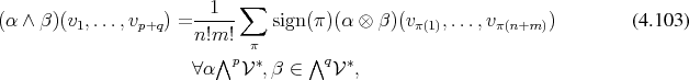
 are permutations of the input vectors and
  is the sign of a permutation.
After the basic geometric entities have been introduced in a per point nature it is desirable to also provide notions of distributed geometric items.
Definition 61 (Scalar field) A smooth mapping  assigning to each point
  of a differentiable
manifold
of a differentiable
manifold  (Definition 37) a value of
  is called a scalar field,

Recalling that charts are bijections (Definition 24), it is possible to pull the scalar field  back (Definition 44) to open sets of
  using
using

 by requiring continuity on
  .
Similarly, differentiability of the scalar field
.
Similarly, differentiability of the scalar field  is defined by demanding the existence of the partial
derivatives of the coordinate functions
is defined by demanding the existence of the partial
derivatives of the coordinate functions  .
.
The scalar fields on  together with the binary operations of addition and multiplication form a ring
 (Definition 13) or
  for short over the manifold.
Using the scalar fields  it is possible to define a derivation (Definition 27)

 .
.

As scalar values are now associated to a manifold  as well as a means of to derive vectors from the
scalar fields, it is also desirable to extend this concept to vectors.
as well as a means of to derive vectors from the
scalar fields, it is also desirable to extend this concept to vectors.
Definition 62 (Vector field) A vector field is defined as a mapping assigning to each point  a
vector from the tangent space
a
vector from the tangent space  (Definition 48) at

Thus any vector field is a section (Definition 41) of the tangent bundle (Definition 52).
Where a vector has been introduced as a mapping of the form  , a vector field is a mapping
of the form
, a vector field is a mapping
of the form  . Thus a vector field appears as a derivation (Definition 27) of scalar field
giving rise to the new scalar field
. Thus a vector field appears as a derivation (Definition 27) of scalar field
giving rise to the new scalar field  :
:

 , which indeed maps back to the scalar fields
  , is said to be differentiable.
Having established the concepts of both differentiable curves (Definition 46) and vector fields (Definition 62) it is possible to link them.
Definition 63 (Integral curves (of vector fields)) A vector field  (Definition 62) on a manifold
 (Definition 37) assigns a vector
  to each point
  . Considering this vector
  as a representative of the differential of a curve
  (Definition 46) at
  defines a set of integral curves
or streamlines of the vector field
defines a set of integral curves
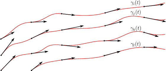
or streamlines of the vector field  as illustrated in Figure 4.5.

The existence of integral curves of a vector field allows to further qualify a vector field, since it links the extended entity of a curve to the local entity of a vector.
Definition 64 (Complete vector field) A vector field  (Definition 62) is said to be
complete, if the integral curves (Definition 63), which are initially only defined locally
(Definition 62) is said to be
complete, if the integral curves (Definition 63), which are initially only defined locally
 , can be extended to all parameters
  for all points
  .
.
Now that vector fields and curves have been intrinsically connected to each other, it is prudent to
reexplore the issue of differing parametrization. Given two curves  and
and  with identical images in
the manifold
with identical images in
the manifold  but differing parametrization


 such as reparametrizations of the form
  do
not change the obtained tangent vectors.
do
not change the obtained tangent vectors.
Similar to vector fields, it is also possible to associate a tensor to every point of a given manifold, thus leading to the next definition.
Definition 65 (Tensor field) A tensor field is defined as a mapping assigning to each point  a
tensor from the tangent tensor algebras
a
tensor from the tangent tensor algebras  (Definition 56) at

Considering a vector field  on a manifold
  defines a system of integral curves, which completely
fill the manifold without intersecting.
defines a system of integral curves, which completely
fill the manifold without intersecting.
Definition 66 (Local flow) The integral curves of a vector field (Definition 63) give rise to a mapping

 and describes a displacement of all points along the local integral curves,
shown in Figure 4.5. This so called flow is considered local, when the mapping is defined for a limited
range of the parameter
and describes a displacement of all points along the local integral curves,
shown in Figure 4.5. This so called flow is considered local, when the mapping is defined for a limited
range of the parameter  . It may also be written as

Where the previous definition was only concerned with local properties, an extension to global scale is possible as well.
Definition 67 (Global flow) A local flow (Definition 66) resulting from a complete vector
field  (Definition 64) and therefore an unconstrained parameter
 ![t ∈ [− ∞; ∞ ]](whole458x.png) is called a
global flow or simply flow.
is called a
global flow or simply flow.
A global flow is a fibration (Definition 39) of the manifold  on which it is defined along
one-dimensional, non-intersecting sub manifolds, the integral curves (Definition 63) of the associated
vector field (Definition 62).
on which it is defined along
one-dimensional, non-intersecting sub manifolds, the integral curves (Definition 63) of the associated
vector field (Definition 62).
Flows and vector fields correspond to each other bijectively (Definition 24): each vector field may be viewed as generating a field by its integral curves, while the corresponding vector field is recovered from a given flow by differentiation. Furthermore, flows can be combined

 with a group structure (Definition 11) where the identity element
is
with a group structure (Definition 11) where the identity element
is

Flows may also be combined with functions  on the manifold
  .
.
The structure of flows will prove to be of importance in further considerations in Section 5.3. It is therefore prudent to further explore relations of flows. As has already been established flows and vector fields (Definition 62) are linked by differentiation, whereby similar structures instantiating Definition 27 become apparent.
A flow  (Definition 67) defines a pull back (Definition 44) of the tensor fields on the manifold
 (Definition 37)

 , which is invariant under a flow

Definition 68 (Lie derivative) The measure of non-invariance of a tensor field with respect to the effect to the pull back due to a flow is obtained by the Lie derivative which is defined as
 is the vector field (Definition 62) generating the flow
  (Definition 67).
In the case of functions, which are represented as tensors of class  , the Lie derivative
yields
, the Lie derivative
yields

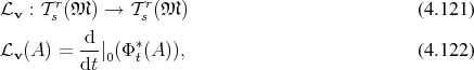
Since the special case of vector fields (Definition 62) is often encountered, it is awarded special notation, which shall not go omitted here, as it will also be used, especially in Chapter 5, which deals with dynamics.
Definition 69 (Lie bracket) The Lie derivative (Definition 68), in the case of vectors, which are
included in Definition 68 as  tensors, is used to define the Lie bracket, also known as the Jacobi
bracket or commutator, as:
tensors, is used to define the Lie bracket, also known as the Jacobi
bracket or commutator, as:
![ℒv(w ) = [v, w ] (4.124)](whole477x.png)
The Lie bracket is skew-symmetric
![[v, w ] = − [w, v] (4.125)](whole478x.png)
![0 = [[v,w ],u] + [[u,v ],w ] + [[w, u ],v]. (4.126)](whole479x.png)
![[v, w ] = 0, (4.127)](whole480x.png)
 and
and  are said to commute. Figure 4.6 gives a visualization of the commutator.
Depending on the order in which the integral curves are followed, either the point
are said to commute. Figure 4.6 gives a visualization of the commutator.
Depending on the order in which the integral curves are followed, either the point  or the point
  is
reached, only in case the vector fields commute, the figure is closed at the point
is
reached, only in case the vector fields commute, the figure is closed at the point  , otherwise, the Lie
bracket yields by how much the closure falls short.
, otherwise, the Lie
bracket yields by how much the closure falls short.
Furthermore, there is a relation between the Lie bracket and the Lie derivative.
![ℒ [v,w] = [ℒv, ℒw ] = ℒvℒw − ℒw ℒv (4.128)](whole490x.png)
The connections of flows with vectors and the Lie derivative enables the definition of an exponential
function  using the following characteristics
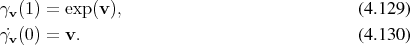

 the following expression can be
established:
the following expression can be
established:

Where the Lie derivative (Definition 68) is specially connected to flows and is a map among tensors (Definition 54) of the same type, mappings among different types of tensors and forms are also needed. They are presented in the following along with their connection to the Lie derivative.
A mapping especially important among  -forms (Definition 59) is provided in the following form of:
Definition 70 (Exterior derivative) A mapping

 -forms to
  -forms with the following properties
 is linear.
 is the differential for smooth functions
  .
.
 –
–  is nilpotent.
 –
–  obeys a graded Leibniz rule.
is called the exterior derivative. It is a (anti)derivation of degree 1.
While the exterior derivative has special importance to forms (Definition 59), a mapping only involving mixed tensors is also useful.
Definition 71 (Contraction) Given a tensor  (Definition 54) for
  the contraction
 is defined as a linear map

 .
.
As a particular special case the contraction can be used to express the scalar product given by
Equation 4.70. Given a vector  and a 1-form
  the scalar product of these two entities can
be expressed using the tensor product (Definition 55) and the just introduced contraction
as
the scalar product of these two entities can
be expressed using the tensor product (Definition 55) and the just introduced contraction
as

 , whose contraction is of type
  which
corresponds to scalar values.
which
corresponds to scalar values.
Where this contraction is defined to act on a single tensor of mixed type, it is also possible to provide a similar and explicit mapping of forms involving an explicitly provided vector field (Definition 62).
Definition 72 (Interior product) Given a vector field  (Definition 62) on a manifold
 (Definition 37) a linear mapping of the form

 is called the interior product.
Written in component vectors it takes the shape:

 -forms it takes the simple form:

The interior product has similar properties to the exterior derivative (Definition 60)  such as
antisymmetry
such as
antisymmetry


 -form
-form  and a
and a  -form
-form
 .
.

 .
.
With the given properties the Lie derivative (Definition 68), the exterior derivative (Definition 70), and the interior product (Definition 72) can be linked in the expression

The exterior derivative allows to qualify differential forms (Definition 59), where the nomenclature is provided in the following definitions.
Definition 73 (Closed form) A form  (Definition 59) with vanishing exterior
derivative (Definition 70)
(Definition 59) with vanishing exterior
derivative (Definition 70)

Definition 74 (Exact form) A form  (Definition 59) is called exact, if it can be expressed by the
external derivative (Definition 70) of another form
(Definition 59) is called exact, if it can be expressed by the
external derivative (Definition 70) of another form 

From the nilpotence of  it follows that every exact form (Definition 74) is closed.
Having established definitions for all components required for the treatment of geometrical problems, they are now assembled into the final settings used for the considerations, which are due to their importance specially named.
The further qualification of differentiable manifolds (Definition 37) is by pairing them with specific tensor fields (Definition 65).
Definition 76 (Metric tensor field) A tensor field (Definition 65) comprised entirely of metric tensors (Definition 75) is called a metric tensor field.
The availability of a metric tensor field allows to define the following:
Definition 77 (Inner product) A metric tensor field  on a differentiable manifold (Definition 37)
defines a non-degenerate bilinear mapping
on a differentiable manifold (Definition 37)
defines a non-degenerate bilinear mapping
for the tangent space at every point. This mapping is called the inner product on the manifold
 .
.
Equipping a manifold with an inner product, defines the notion of orthogonality of two vectors in the tangential spaces at each of the points. This structure is of such significance, it warrants the following definition.
Definition 78 (Riemannian manifold) The pair  of a differential manifold
 (Definition 37) on which a positively definite metric tensor field
  (Definition 76) is
defined and hence an inner product is available, is called a Riemanninan manifold.
(Definition 76) is
defined and hence an inner product is available, is called a Riemanninan manifold.
Riemannian manifolds carry sufficient structure to define angles between vectors in each of the tangential spaces, but also allows for the definition of the concept of how far any two points of the manifold are apart, which is explored further in Section 4.8.
A Riemannian manifold, where all tangent spaces (Definition 48) are identical and which can therefore be covered by a single chart (Definition 36), is a very important special case encountered in everyday perception and has been the foundation of important developments in physics, as illustrated in Section 5.1.
In this case the structure can be simplified considerably, as can be experienced in the following two definitions.
Definition 79 (Affine space) A set of points  accompanied by a vector space
  (Definition 16) is
called an affine space, if the following assertions hold:
(Definition 16) is
called an affine space, if the following assertions hold:
 to an element
  exists.
 and vector
  there is exactly one point
  such
that
such
that

 it holds

 is called the tangent space of
  .
.
The nomenclature in the case of the affine space is reminiscent of the manifold, however, the previously locally varying structures are now constant over all of the considered space. With these requirements an affine space inherently supports the notion of parallel lines. It however lacks structure to define lengths and angles.
Adding the structure of an inner product (Definition 77) remedies this deficiency and results in:
Definition 80 (Euclidean space) An affine space (Definition 79), where the tangent space
 (Definition 48) is equipped with an inner product which defines a norm, is called an
Euclidean space
(Definition 48) is equipped with an inner product which defines a norm, is called an
Euclidean space  .
.
Similarly to the symmetric metric structure (Definition 76) yielding the concepts of length and angles, a skew-symmetric structure has a distinct application as is illustrated in Section 5.3. The required structure begins by a simple definition.
Definition 81 (Symplectic form) A non-degenerate, closed (Definition 73), skew-symmetric
bilinear form  is called a symplectic form.
This definition is now used to qualify a manifold similarly to the Riemannian (Definition 78) case.
Definition 82 (Symplectic manifold) The pair  of a differentiable manifold
 (Definition 37), where a symplectic form
  is defined in every tangent space
  , is
called a symplectic manifold.
, is
called a symplectic manifold.
Due to the non-degeneracy together with the demand of skew-symmetry all symplectic manifolds necessarily have even dimension.
Definition 83 (Symplectic map) A diffeomorphism (Definition 38)

 and
and  are symplectic
manifolds (Definition 82). The symplectic form can be expressed as a pullback (Definition 44).
are symplectic
manifolds (Definition 82). The symplectic form can be expressed as a pullback (Definition 44).

Connected with symplectic spaces is an important theorem regarding the representation of the symplectic form. It is the basis for canonical representations in Section 5.3.
Definition 84 (Darboux’s theorem) Given a  -dimensional symplectic manifold
 (Definition 82) the symplectic form
  (Definition 81) can always be rendered in the
canonical form
(Definition 81) can always be rendered in the
canonical form
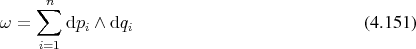
 for every point
  .
.
Definition 85 (K¨ahler manifold) A complex manifold  which has both a Riemannian and
symplectic structure is called a K¨ahler manifold. It is required that the metric structure
which has both a Riemannian and
symplectic structure is called a K¨ahler manifold. It is required that the metric structure  and
symplectic structure
and
symplectic structure  are compatible in the following manner:

 composed as

The existence of a non-degenerate bilinear form, metric (Definition 76) or symplectic (Definition 81),
allows to define an isomorphism between the tangent and co-tangent bundles of a manifold. This is
accomplished by associating to every vector  tangent to
  at a point
  one form
by
one form
by


 defines a
  -form and is thereby linked to it, defining an
isomorphism.
-form and is thereby linked to it, defining an
isomorphism.

 -form. The existence of such a mapping is essential as it also provides a structure with
which to translate different kinds of tensors into one another.
-form. The existence of such a mapping is essential as it also provides a structure with
which to translate different kinds of tensors into one another.
Furthermore it is possible to identify flows and their associated vector fields which preserve the metric or symplectic structures. Using the Lie derivative this reads

 . The vector fields meeting this requirement are called Killing vector
fields [74 ]. In the symplectic case the expression is almost identical with the symplectic form taking the
place of the metric
. The vector fields meeting this requirement are called Killing vector
fields [74 ]. In the symplectic case the expression is almost identical with the symplectic form taking the
place of the metric


 is closed and hence
  , it follows


 is a function on the symplecetic manifold
  . The function
  generates the vector field
  .
The definition of
.
The definition of  in Equation 4.161 is implicit and may be converted to an explicit form using the
isomorphism defined in Equation 4.156 to obtain
in Equation 4.161 is implicit and may be converted to an explicit form using the
isomorphism defined in Equation 4.156 to obtain

Definition 86 (Poisson bracket) The Poisson bracket is obtained by applying the Lie bracket for vector fields to an expression due to the established isomorphism (Equation 4.156).
![[Idf,Idg ] = [vf ,vg] = v{f,g} (4.163)](whole606x.png)
 is a bilinear, skew symmetric map
satisfying the Jacobi identity.
is a bilinear, skew symmetric map
satisfying the Jacobi identity.
A manifold  along with a Poisson structure is called a Poisson manifold. Every symplectic manifold
is also a Poisson manifold, while the reverse is not necessarily true, as the Poisson structure may be
degenerate, thus being more general. In the symplectic case, the Poisson structure and the symplectic
structure are inverse to each other.
along with a Poisson structure is called a Poisson manifold. Every symplectic manifold
is also a Poisson manifold, while the reverse is not necessarily true, as the Poisson structure may be
degenerate, thus being more general. In the symplectic case, the Poisson structure and the symplectic
structure are inverse to each other.

| | |
![κ ∘ γ : I → ℝn (4 .64a)
i
x (s) : I → ℝ,∀i ∈ [0,...,n − 1] (4.64b)](whole295x.png)


 .
. 


 of a vector field.
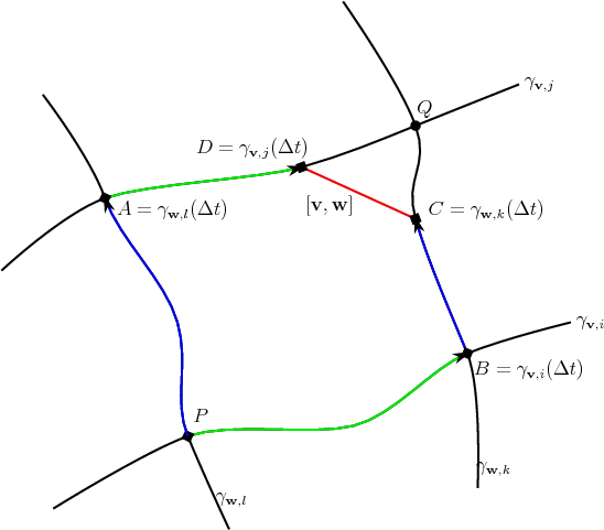
![[v, w ]](whole487x.png) of two vector fields
of two vector fields  and
and  .
.