The Quantum World

5.7 The Quantum World

While mechanics in its classical form describes the world with determinism, even if predictability is undermined, when turning to statistical methods, this is drastically changed in a quantum mechanical setting. Already well established and tangible concepts such as particles are recast in the setting of quantum mechanics using wave functions. This makes eﬀects describable, which are completely unavailable to the classical setting, without changing the Newtonian structure of the universe with its absolute time.

Quantum mechanics is often introduced in a detached manner with little to no connection to the classical settings supporting utterly alien eﬀects which even border on the bizarre. It is therefore interesting to note that the governing structures so painstakingly uncovered by scientists over the course of time for the classical case are still present in the quantum setting. This comes as no surprise in light that the macroscopic world of every day life follows classical rules, wherefore the descriptions of quantum systems should always yield classical behaviour, when taken to the appropriate limit.

The setting of the quantum world is chosen to be a complex Hilbert space from which functions are chosen to represent the state of a system. The structure of this complex Hilbert space together with a link to the macroscopic world is suﬃcient to extract the governing equation of the system.

The wave functions $Ψ$ , which are drawn from the complex Hilbert space $ℋ$ are acted upon mappings, which are often called operators in this context, to describe transitions of states. While the $Ψ$ are capable of encoding the state of a quantum system, they elude observations completely. At ﬁrst this seems to contradict the requirement that scientiﬁc theories must be falsiﬁable [93] and thus accessible to some form of experiments and measurement. However, observables can be constructed from $Ψ$ in a systematic fashion, which are again accessible to measurements and thus to testing of the theory. Without touching upon the, for many researchers sensitive, topic of the many diﬀerent interpretations of quantum mechanics [94][95][96][97] the wave functions $Ψ ∈ ℋ$ need to meet the following property

⟨Ψ |Ψ ⟩ = 1 (5.52)

as to allow the interpretation as a probability.

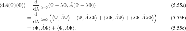
The prescription of constructing observables yields expectation values (Deﬁnition 101) of previously classically determined entities such as location or momentum. It is thus a reasonable demand that this mapping shall produce entities with their expected structures, e.g., appropriate tensors (Deﬁnition 54).

A : ℋ → T r (5.53) s

In this fashion a correspondence of operators acting on $Ψ$ and classical observables is established

⟨A ⟩ = ⟨A(Ψ )⟩ = ⟨Ψ|Aˆ|Ψ ⟩, (5 .54)

where $⟨A⟩$ is the classical expectation value (Deﬁnition 101) and $Aˆ$ is a operator on elements of the Hilbert space. This deﬁnes the observable operators on $Ψ$ .

As in the classical case, a diﬀerential form (Deﬁnition 59) is derivable with a function $A$ on the Hilbert space $ℋ$ . At a point $Ψ ∈ ℋ$ for a tangent vector $Φ$ (Deﬁnition 48) using an arbitrary parameter $λ$ this gives

d ⟨dA(Ψ)(Φ )⟩ = ---|λ=0⟨Ψ + λΦ, ˆA(Ψ + λΦ )⟩ (5.55a) dλ ( ) = d--| ⟨Ψ, ˆAΨ ⟩ + ⟨Ψ,AˆλΦ ⟩ + ⟨λΦ,AˆΨ ⟩ + ⟨λ Φ,AˆλΦ ⟩ (5.55b) dλ λ=0 = ⟨Ψ, AˆΦ ⟩ + ⟨Φ, ˆAΨ ⟩. (5.55c)

In case $ˆ A$ is self adjoint with respect to the scalar product, this can be reshuﬄed to

⟨AˆΨ, Φ⟩ + ⟨Φ, ˆAΨ ⟩. (5.56)

Since a complex Hilbert space $ℋ$ is also a K¨ahler space (Deﬁnition 85), the Hermitian inner product (Deﬁnition 77) of $ℋ$ may be rendered as a composition of a Riemannian component $g$ (Deﬁnition 76) and a symplectic component $ω$ (Deﬁnition 81).

1 1 h(x, y) = ---g(x,y) + ---ω(x, y) (5.57) 2ℏ 2ℏ

Thus the preceding expression may be modiﬁed to

-1- ˆ -1- ˆ 1- ˆ 2ℏ g(AΨ, Φ ) + 2 ℏg(Φ, AΨ ) = ℏ g(AΨ, Φ ), (5 .58)

from which, due to the relation between symplectic and Riemannian part as required by the K¨ahler structure, it follows further

1g(AˆΨ, Φ) = − i-ω(AˆΨ,Φ ). (5.59) ℏ ℏ

Which motivates, in allusion to the Hamiltonian vector ﬁelds (Deﬁnition 62) of the classical case, the association of a Hamiltonian vector ﬁeld $v ˆAΨ$ with an operator $Aˆ$ by

vˆ(Ψ ) = − iAˆΨ, (5 .60) A ℏ

which ﬁnally enables to conclude using the interior product (Deﬁnition 72)

⟨dA(Ψ )(Φ)⟩ = ω (vˆAΨ,Φ ) = (ivˆAΨω)(Φ ). (5.61)

As can be observed, the classical expectation value can be linked to the symplectic structure inherent to the complex Hilbert space $ℋ$ .

Thus the structures governing the evolution of the classical case, in the form of Hamiltonian vector ﬁelds, are also recognizable in a quantum system. While all of the Hilbert space is endowed with the symplectic structure, the normalization requirement conﬁnes the selection of states to the unit hyper-sphere. However, this restriction is not suﬃcient to remove all ambiguity, since it still remains in the form of uni-modular factors

Ψ′ = cΨ, |c| = 1. (5.62)

This remaining ambiguity is removed by further restricting the Hilbert space to a projective space $ℋ𝒫$ . This projective space may now be regarded as a phase space connected to a physical system.

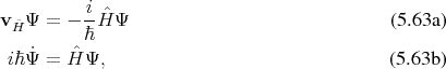
In case of the Hamiltonian operator, the prescription 5.60 of assigning vector ﬁelds to operators yields exactly Schr¨odinger’s equation as can be seen by

vˆΨ = − i-ˆH Ψ (5.63a) H ℏ iℏΨ˙ = HˆΨ, (5.63b)

which is the main governing equation of the quantum system. Thus the Hamiltonian vector ﬁeld deﬁned in this fashion is indeed responsible for the evolution of the quantum system in the Schr¨odinger picture of quantum mechanics, where operators remain constant and the states evolve.

While a function $Ψ ∈ 𝒫 ℋ$ captures a state completely, descriptions usually employ a representation using either position $r$ or momentum $p$ representations, which may be obtained by (utilizing Bra-Ket notation introduced in Section 4.6.2)

Ψ (r,t) = ⟨r|Ψ (t)⟩ (5.64)

and

Φ(p, t) = ⟨p |Φ (t)⟩. (5.65)

The change between these two representations is possible using a Fourier transform

n ∫ i Φ(p, t) = (2π ℏ)−2 Ψ (r,t)e−ℏ⟨p,r⟩dr (5 .66a) ∫ − n2 iℏ⟨p,r⟩ Ψ (r,t) = (2π ℏ) Φ (p,t)e dp, (5.66b)

where $n$ is the spatial dimension of the problem under investigation.

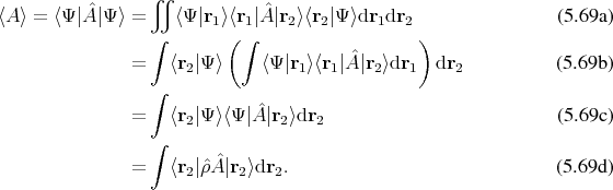
These descriptions account for half the degrees of freedom implicitly, while exposing only the other half. It is, however, possible to construct a representation, which explicitly recovers all degrees of freedom. The density operator and the density matrix are such representations. The density operator is given by

ρˆ= |Ψ ⟩⟨Ψ|. (5.67)

By evaluating this operator at two diﬀerent positions in the form

∫ ρ(r1,r2) = ⟨r1|ρˆ|r2⟩ = ⟨r1|Ψ⟩⟨Ψ |r2⟩ = Ψ ∗(r2)Ψ (r1) (5.68)

the density matrix $ρ(r1,r2)$ is obtained, which may be seen as a measure of correlation between two positions $r1$ and $r2$ and retains all state information encoded in $Ψ$ , as may be reinforced when reformulating Equation (5.54) as

∬ ⟨A ⟩ = ⟨Ψ|Aˆ|Ψ ⟩ = ⟨Ψ|r1⟩⟨r1|A ˆ|r2⟩⟨r2|Ψ ⟩dr1dr2 (5.69a) ∫ ( ∫ ) ˆ = ⟨r2|Ψ ⟩ ⟨Ψ |r1⟩⟨r1|A |r2⟩dr1 dr2 (5.69b) ∫ = ⟨r2|Ψ ⟩⟨Ψ |A ˆ|r2⟩dr2 (5.69c) ∫ = ⟨r2|ρˆˆA|r2⟩dr2. (5.69d)

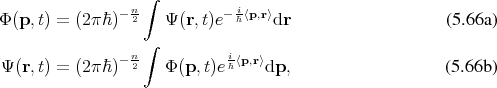
Utilizing such a representation, which provides information about the correlation of all of the points in the problem domain, it is possible to also construct a representation which uses the position $r$ and the momentum $p$ , or wave vector $k$ associated by

p = ℏk, (5 .70)

to describe the quantum system and thus mapping it to a phase space similar to the classical settings. This is provided by the so called Wigner-Weyl transform [98][99], where the Wigner transform of an operator is given by

∫ ∞ r r i A (q, p) = ⟨q − -| ˆA|q +--⟩e−ℏ⟨p,r⟩dr (5.71) − ∞ 2 2

In the case of the density operator, a quasi-probability distribution function $f$ is obtained,

∫ ∞ r r − i⟨p,r⟩ f(q, p) = ⟨q − --|ρˆ|q + -⟩e ℏ dr, (5 .72) −∞ 2 2

which mirrors the distribution function of the classical case but, is no longer positively deﬁnite and thus can not be strictly interpreted as a probability density function, since it is no longer a measure but a signed measure (Deﬁnition 91). It is, however, possible to compute expectation values (Deﬁnition 101) in the usual manner using

∫ ⟨X ⟩ = Xf dqdp (5.73)

for a quantity $X$ .

Since the transform linking the representations in terms of $ρ$ and $f$ is linear, the evolution of the system may be expressed in either of them equivalently. The structures inherent to the space of quantum mechanics also allow to formulate the evolution of a physical quantity, such as for the $ˆρ$ as

[ ] ˆρ˙= ρˆ, ˆH + ∂-ˆρ, (5 .74) ∂t

which takes on a similar shape in the quantum phase space using the quasi-probability distribution function. It has to be noted, however, that the Lie bracket (Deﬁnition 69) applied in the context of operators in the Hilbert space has a slightly warped shape in the quantum phase space, due to the transformation given in Equation 5.71. The deformation takes on the form [100]

( ) {f,g}M = 2-sin ℏ- -∂--∂- − -∂- ∂-- f(q, p)g(q,p ). (5.75) ℏ 2 ∂q ∂p ∂p ∂q

Using this deformed bracket, the evolution in quantum phase space can be described as

∂ f˙= {f, H }M + --f, (5 .76) ∂t

which mimics the classical case as expressed in Equation 5.31. It also follows that the classical Poisson bracket and hence classical evolution can be recovered from the prescription given in Equation 5.75 in the limit $ℏ→0$ , thus this construct meets a basic property demanded from a quantum description.