| | |
Where many concepts and notions are defined in a purely local fashion, others, such as expectation values (Definition 101) or distances (as presented in Section 4.8), have a non-local nature which is accounted for by utilizing integrals for their description. In many cases the determination of the result of integration can make use of the fundamental theorem of calculus or its generalization of Stokes’s theorem.When this is to be used to obtain a value connected to the integrated expression, it relies on the result being expressible in the limited terms of elementary functions, which, unfortunately, severely limits the range of applicability. For this reason several alternate methods which are not limited by elementary functions have been developed.
A possible venue to provide a means of evaluating integrals which do not match an elementary function, is by using approximations based on selected elementary functions to calculate the value of the integral. Different strategies, sharing the approach of relying on polynomials (Definition 19) and their properties have been developed, since polynomials are not only very adaptable, but also easy to integrate, as the polynomial functions are closed under integration. Common to all of these methods is that an estimate for the integral is obtained by sampling the integrand at several discrete points obtained by subdivision of the integration domain.
A simple strategy is to approximate the integrand directly by constructing an approximate polynomial which is then integrated. In order to avoid high orders of polynomials, which have proven to be numerically problematic, local approximations of low polynomial order can be used. Following this idea using equidistant subdivisions leads to the Newton-Cotes method. The use of different degrees of polynomials for local approximation leads to rectangular, trapezoid, and quadratic estimates.
It should not go without notice that it is possible to construct schemes of higher order by using linear polynomials, which give rise to the trapezoid quadrature procedure. This is accomplished by applying Richardson extrapolation (see Appendix C) to the trapezoid quadrature to improve its accuracy and is known as the Romberg method, Romberg rule or Romberg quadrature. By repeating the application of Richardson extrapolation, it is possible to obtain a quickly converging algorithm, which furthermore allows for the reuse of previously computed values. The fast convergence of the algorithm, however, relies on the existence of derivatives of an order corresponding to the order of approximation.
A different approach for efficient quadrature turn to utilizing orthogonal polynomials, to derive a
different method of numerical integration, which is known as Gauß quadrature. It draws on the
properties of orthogonal polynomials to precompute weighting coefficients  associated with
positions
associated with
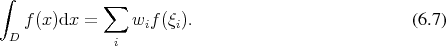
positions  to formulate the integral as
Several variants of all of these algorithms have been developed, as well as methods differing in their particulars, but using the same approaches [116], resulting in a selection of numerical integration schemes from which to choose. There is, however, no best method of quadrature in general, especially if there is no a priori knowledge if the integrand. Thus the creation of options from which to choose from is of high importance in this field. This has proved to be a set of powerful tools in one dimension, however, as the dimension of the integral increases, these methods become less attractive, due to an exponential increase in required sampling points and function evaluations [117] to maintain quality of approximation, which drastically increases the computational burden. Therefore, alternatives to these methods should also be considered, if multi-dimensional integration is required or desired.
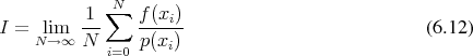
A different approach to the subject of integration, which does not deteriorate as the dimension of the integration domain increases has also been developed. The stochastic nature of the procedure has earned it the name of Monte Carlo method [118][119][120][121][122][123]. Since it is not easily possible to evaluate multi-dimensional integrals by simple deterministic methods described in Section 6.6.1. Monte Carlo methods provide a simple and elegant solution which becomes increasingly attractive as the dimensionality of the integration domain increases. The task of determining the value of a given integral (Definition 94)
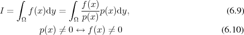
 is viewed as a probability density function (Definition 100).
For
is viewed as a probability density function (Definition 100).
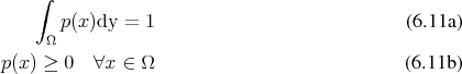
For  to be considered a probability density, it has to meet the following restrictions.
The reinterpretation as an expectation value (Definition 101) in conjunction with a probability density also provides an intuitive way for moving from the continuous realms of the initial problem domain to a discrete one, such as present in digital computers.
Calling on the law of large numbers, it is possible to relate several discrete realizations modelled after
the probability density  sampling the integration domain
  to the expectation value
  as the
sample mean approaches the expectation value.
as the
sample mean approaches the expectation value.
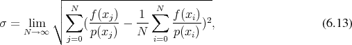
 does not depend on the choice of the distribution
function. The variance
does not depend on the choice of the distribution
function. The variance
 using the three
  rule, which ensures that the true value of the integral lies
within the interval of
rule, which ensures that the true value of the integral lies
within the interval of  with a probability of
  percent.
Using the C++ programming language and relying on already available libraries [109] the central part of the implementation of a Monte Carlo integrator may be accomplished in a very concise manner, as the next listing of code demonstrates.
It uses the boost::accumulator library to conveniently keep track of the mean of the evaluated points, thereby constructing an estimator for the true value of the integral under consideration. This estimator contains the mean value, which is the main estimate along with the corresponding statistical error. The library’s facilities make it simple to realize this behaviour by simply specifying the corresponding tags, boost::accumulators::tag::mean and boost::accumulators::tag::error_of<> respectively. Furthermore, it requires a source of random variables (see Appendix B), provided here in the form of random_source. The function to be integrated itself is represented as a function object eval. The estimator is then fed with function evaluations corresponding to a sequence of random numbers.
As can be seen, the dimensionality of the problem does not enter into this implementation explicitly. It is completely encapsulated within the invocation of the eval function object, which relies on an appropriate random number generator.
When considering parallelization of the loop in this code, special care must be taken on the one hand of the estimator, which internally keeps track of the mean value and thus must be handled appropriately. On the other hand, the generation of random numbers in parallel may also result in issues, when left unchecked.
| | |