2.5 Interpolation Method
The available oxidation models alone fail to predict the oxide growth for 3D structures due to their 1D nature. An approach which extends these models by incorporating the crystal direction dependence into the oxidation growth rates has thus been developed [73, 92] and is discussed in the following.
The geometrical aspects of SiC can be mathematically described according to basic crystallography [105] and experimental findings [88, 86]. A unit cell of the hexagonal crystal structure includes six \((1\bar 100)\) m-faces and six \((11\bar 20)\) a-faces symmetric with respect to the z axis, while there is only one \((0001)\) Si-face on the top and one \((000\bar 1)\) C-face on the bottom of the crystal structure.
To obtain the oxidation growth rate for an arbitrary crystal direction, a direction-dependent interpolation method [92] is utilized. This interpolation method computes a growth rate for a given crystal direction based on a set of known growth rate values. The known growth rates have been discussed in the previous section (cf. Section 2.4), i.e., the growth rates of the Si-, m-, a-, and C-face, which correspond to the \((0001)\), \((1\bar 100)\), \((11\bar 20)\), and \((000\bar 1)\) crystal directions, respectively [70, 63, 87]. These four oxidation growth rates are input arguments for the interpolation method.
The interpolation method consists of a symmetric star shape in the x-y plane and a tangent-continuous union of two half-ellipses in z direction. The method yields a symmetry in the x-y plane such that the oxidation growth rates in direction of a- and m-faces repeat six times with an enclosed angle of π/6. A schematic representation of the interpolation in the x-y and x-z plane is shown in Figure 2.14. The blue lines refer to the interpolation between the known growth rates, indicated with the cross symbols. The direction and the length of the arrows represent crystal directions toward SiC faces and oxidation growth rate values, respectively. A less accurate linear interpolation could be considered as well, shown with the dotted black lines and sharp edges, which would also fit the geometry of SiC. However, the non-linear method offers considerable higher accuracy [92]. The interpolation method can be represented in a parametric or an explicit expression. Both approaches are discussed in the following sections.
(a)

(b)
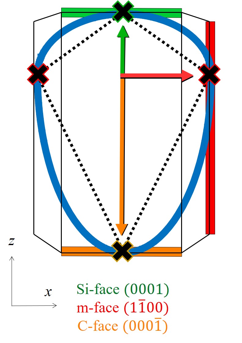
Figure 2.14: Schematic representation of the interpolation method in the (a) x-y and (b) x-z plane. A linear (black dotted) and a non-linear (blue line) interpolation is calculated according to four known growth rate values (black crosses) of Si- (green), m- (red), a- (blue), and C-face (orange square). Colored arrows represent crystal directions towards the corresponding faces. The arrow lengths are proportional to the oxidation growth rates.
2.5.1 Parametric Expression
For plotting surfaces of higher dimensions, the most convenient representation of the interpolation method in 3D space is the parametric expression, written as [73]
\( \seteqsection {2} \) \( \seteqnumber {54} \)
\begin{equation} \begin {split} x&=\left (k_y+(k_x-k_y) \cos ^2(3t)\right ) \cos (t) \cos (u), \\ y&=\left (k_y+(k_x-k_y) \cos ^2(3t)\right ) \sin (t) \cos (u), \\ z&=k_z \sin (u), \end {split} \label {eq:parametric} \end{equation}
where x, y, and z are the Cartesian coordinates, t ∈ [0, 2π] and u ∈ [-π/2, π/2] are the arbitrary parametric variables, and kx, ky, and kz are the oxidation growth rates in directions of x, y, and z, respectively. In this case the following values are considered: kx = km, ky = ka, and kz = kC or kSi.
As shown in several studies [70, 69, 79], the oxide growth on the top and the bottom of the SiC crystal is different, thus the positive and the negative z coordinates are calculated separately, yielding
\( \seteqsection {2} \) \( \seteqnumber {55} \)
\begin{equation} \begin {split} z&=k_z^{+} \sin (u) \mathrm { for } u \geq 0 \mathrm { and} \\ z&=k_z^{-} \sin (u) \mathrm { for } u < 0. \end {split} \label {eq:parametric_z} \end{equation}
kz+ and kz- correspond to the growth rates in the direction of the Si- and C-face, respectively. Thus, it is defined that kz+ = kSi and kz- = kC.
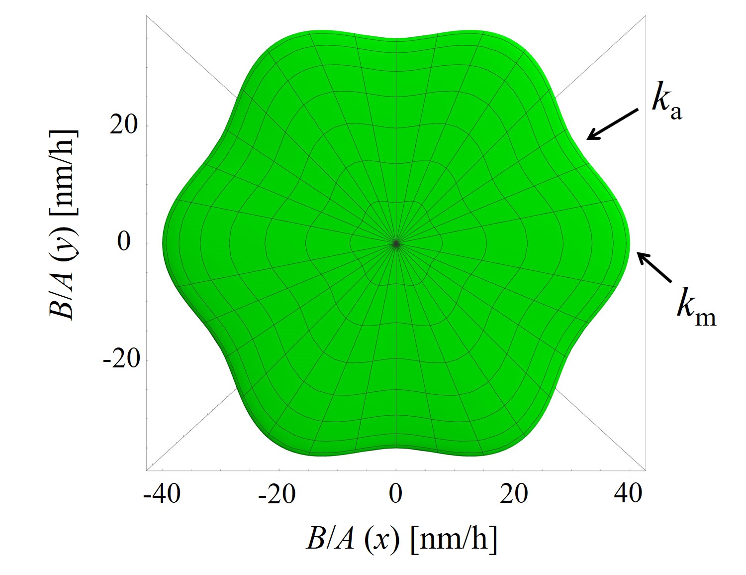
The parametric expression of the interpolation method (2.54) is utilized to calculate, for example, linear oxidation growth rates (B/A) in 3D space, shown in Figure 2.15. Calculations are performed with the known oxidation parameters at T = 1100°C, i.e., kSi = 1.81 nm/h, ka = 35.9 nm/h, km = 41.0 nm/h, and kC = 70.2 nm/h (cf. Section 2.4.2) [72].
The growth rate surface is given by a nonlinear interpolation between these known growth rate values and follows the geometry of SiC, i.e., the crystallographic planes tangent to the growth rate surface at kSi, km, ka, and kC are parallel to the corresponding faces. The distance from the origin (0, 0, 0) to any point on the growth rate surface gives the oxidation rate in direction to this point. For example, if we consider to calculate a single oxidation growth rate in direction of t = 1/4 π and u = 1/4 π, the result according to (2.54) is: k(x) = 19.23 nm/h, k(y) = 19.23 nm/h, and k(z) = 1.28 nm/h. The final oxidation growth rate is the distance from the origin to (x, y, z): (19.232 + 19.232 + 1.282)1/2 nm/h = 27.22 nm/h.
(a)
(b)
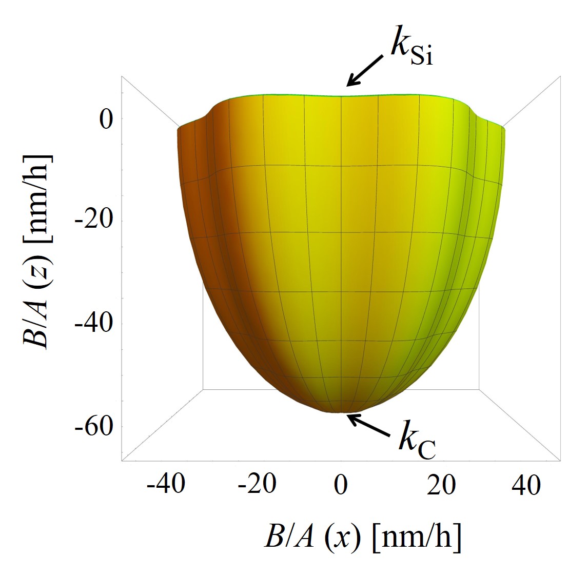
Figure 2.15: 3D calculations of the linear oxidation growth rates B/A obtained with the parametric expression of the interpolation method. The figure shows (a) the top and (b) the front view of the growth rates’ surface. An arbitrary direction growth rate is calculated according to the four known growth rates (kSi, km, ka, and kC) shown with the black arrows. The surface colors show calculations for positive (green) and negative (orange) z direction. The calculations are performed for oxidation at T = 1100°C.
2.5.2 Explicit Expression
The parametric expression of the interpolation method can be converted into an explicit expression, which describes the surface as the zero set of equation f (x, y, z) = 0, where x, y, and z are the vector coordinates of the arbitrary direction of interest. The explicit expression follows the geometry of the hexagonal structure just like the parametric expression, but returns a value in the range from 0 to 1. The explicit expression is thus
\( \seteqsection {2} \) \( \seteqnumber {56} \)
\begin{equation} f(x,y,z) = \Big (2(x^2+y^2)^3 - (x^2 + y^2)^4 - x^2 (x^2 - 3 y^2)^2 \Big ) + z^2. \label {eq:function-inter} \end{equation}
The direction vector \(\vec{v}\)(x, y, z) must be normalized, i.e., vector length \(|\vec{v}|\) = 1. Using expression (2.56), the growth rate coefficients are rewritten into an interpolation method such that [106]
\( \seteqsection {2} \) \( \seteqnumber {57} \)
\begin{equation} \begin {split} k(x,y,z) = k_{y} & + \Big (k_{x} - k_{y}\Big ) \Big (2(x^2+y^2)^3 \\ & \qquad \qquad \qquad - (x^2 + y^2)^4 \\ & \qquad \qquad \qquad - x^2 (x^2 - 3 y^2)^2 \Big ) \\ & + \Big (k_{z} - k_{y}\Big ) z^2. \end {split} \end{equation}
Including the four known growth rate values in the 3D interpolation method and treating the positive and the negative z coordinates separately yields
\( \seteqsection {2} \) \( \seteqnumber {58} \)
\begin{equation} \begin {split} k(x,y,z) = k_\mathrm {a} & + \Big (k_\mathrm {m} - k_\mathrm {a}\Big ) \Big ( 2(x^2+y^2)^3 \\ & \qquad \qquad \qquad - (x^2 + y^2)^4 \\ & \qquad \qquad \qquad - x^2 (x^2 - 3 y^2)^2 \Big ) \\ & + \Big (k_\mathrm {Si} - k_\mathrm {a}\Big ) z^2 \text { for } z \geq 0 \mathrm { or} \\ & + \Big (k_\mathrm {C} - k_\mathrm {a}\Big ) z^2 \text { for } z < 0. \end {split} \label {eq:explicit} \end{equation}
kSi, km, ka, and kC are the four known growth rate values, which correspond to the Si-, m-, a-, and C-face, respectively.
The explicit representation is more general and more suitable for 1D and 2D calculations, because it is more closely related to the concepts of constructive solid geometry and is typically represented with x and y coordinates. However, the parametric form is more convenient for 3D plotting and remains dominant in computer graphics and geometrical modeling due to the ability to reduce the number of independent variables, i.e., it replaces the coordinates x, y, and z with two parametric variables t and u.
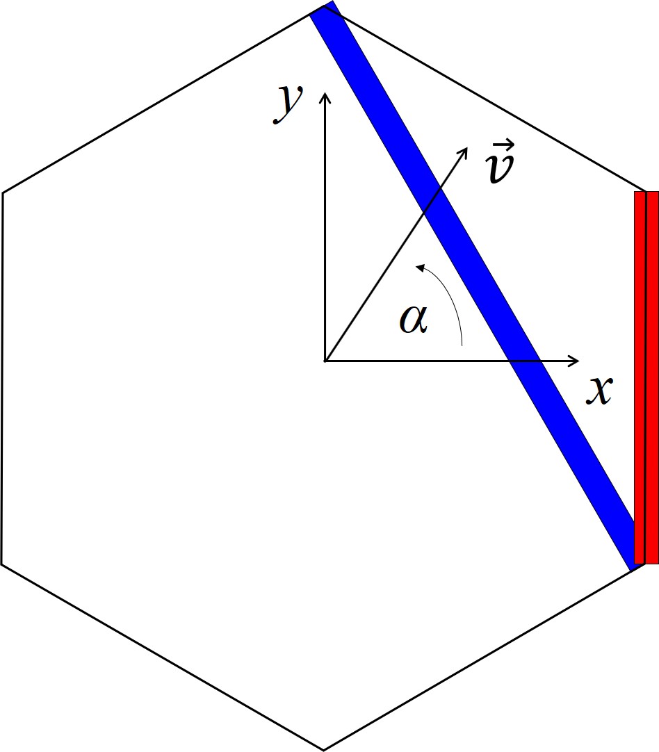
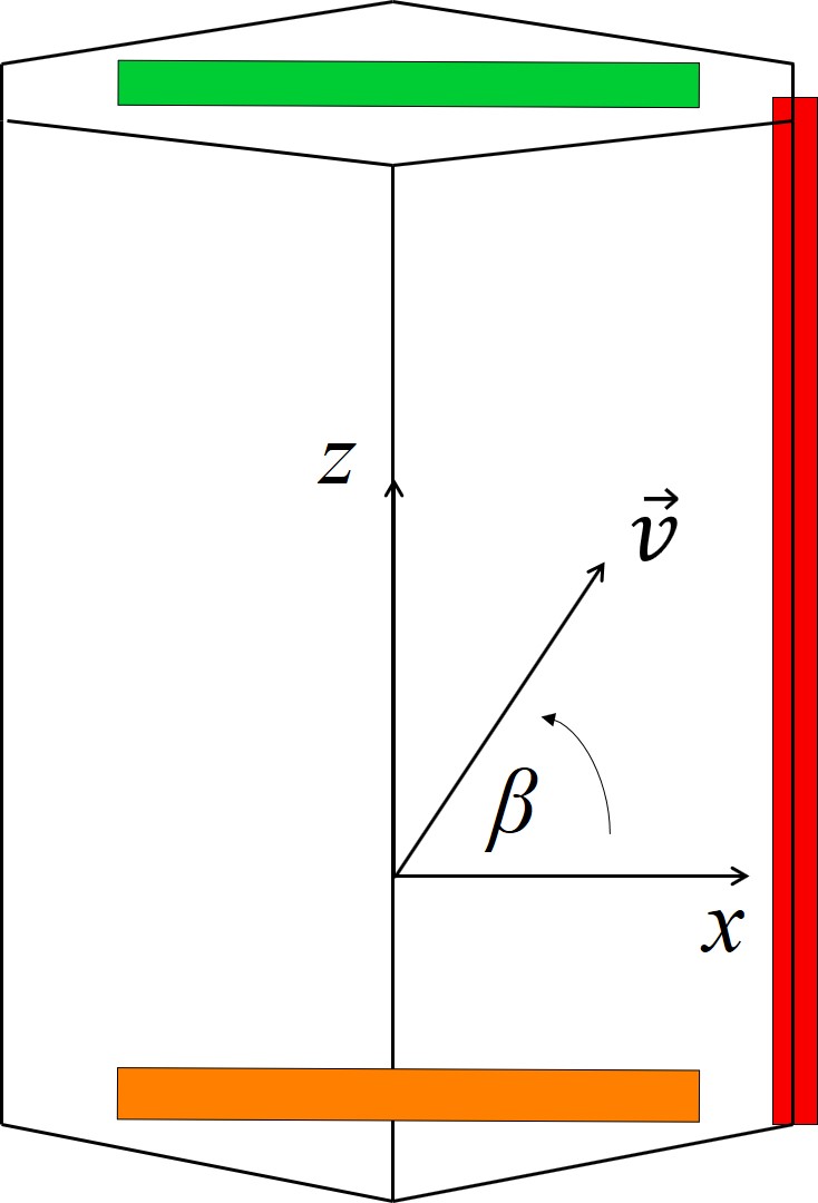
Schematic representations of the hexagonal crystal structure and the variables for the following calculations are shown in Figure 2.16. 2D calculations are typically performed either in the x-y, x-z, or (x+y)/2-z plane. The input of the interpolation method is an arbitrary crystal direction vector \(\vec{v}\) contained in the x-y or x-z plane for which the oxidation growth rate has to be computed. Denoting the angle between \(\vec{v}\) and the x axis by α in x-y plane or by β in x-z plane yields the following relations
\( \seteqsection {2} \) \( \seteqnumber {59} \)
\begin{equation} \begin {split} x =& |\vec {v}| \cos {\alpha }, \\ y =& |\vec {v}| \sin {\alpha }, \end {split} \end{equation}
and
\( \seteqsection {2} \) \( \seteqnumber {60} \)
\begin{equation} \begin {split} x =& |\vec {v}| \cos {\beta }, \\ z =& |\vec {v}| \sin {\beta }. \end {split} \end{equation}
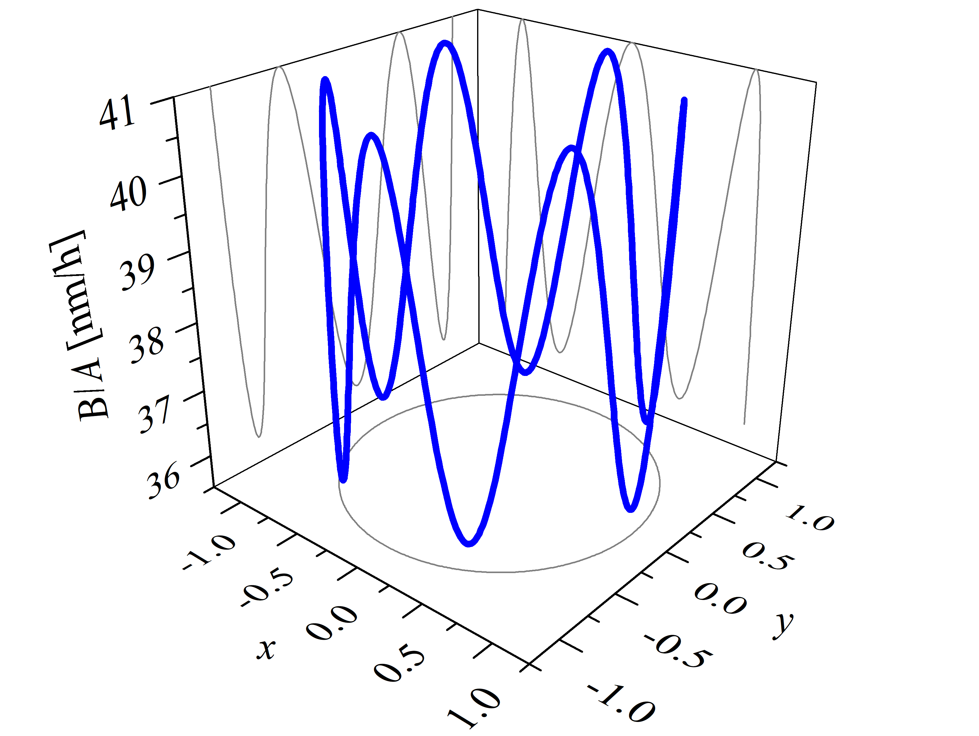
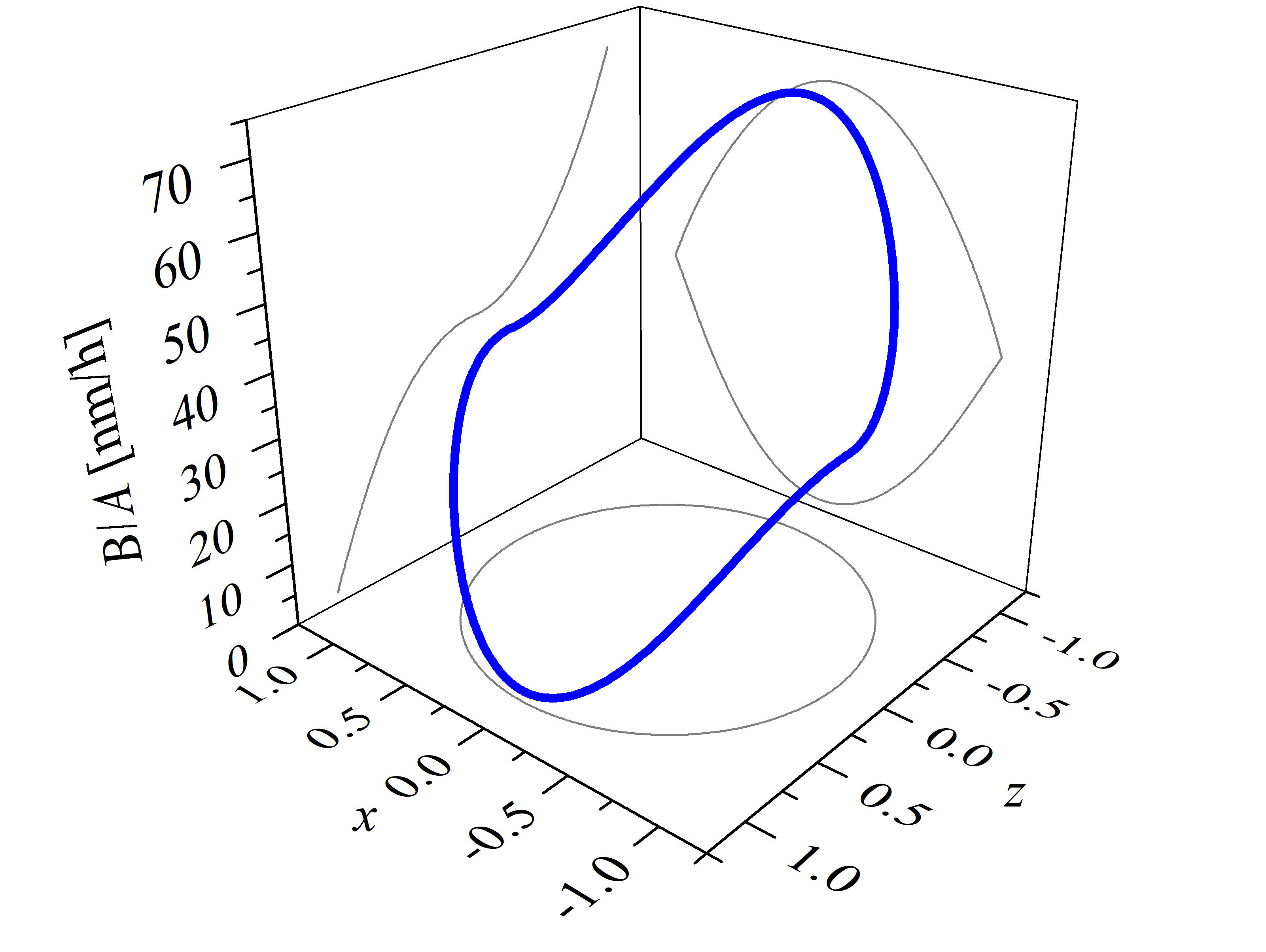
The explicit expression of the interpolation method (2.58) is utilized for calculations of arbitrary oxidation growth rates in 2D space. For example, the linear growth rates (B/A) of the thermal SiC oxidation, shown in Figure 2.17, are calculated with the known growth rate parameters at T = 1100°C, i.e., kSi = 1.81 nm/h, ka = 35.9 nm/h, km = 41.0 nm/h, and kC = 70.2 nm/h (cf. Section 2.4.2) [72]. Calculations are performed in the x-y and x-z plane using normalized crystal direction vector coordinates x, y, and z as input for the interpolation method. The combination of vector coordinates (x, y or x, z) define the crystal direction for which the oxide thickness is calculated. The considered vectors cover the whole x-y and x-z plane of the given crystal directions, which is clearly seen by the gray circle below the plots.
(a)
(b)
(c)
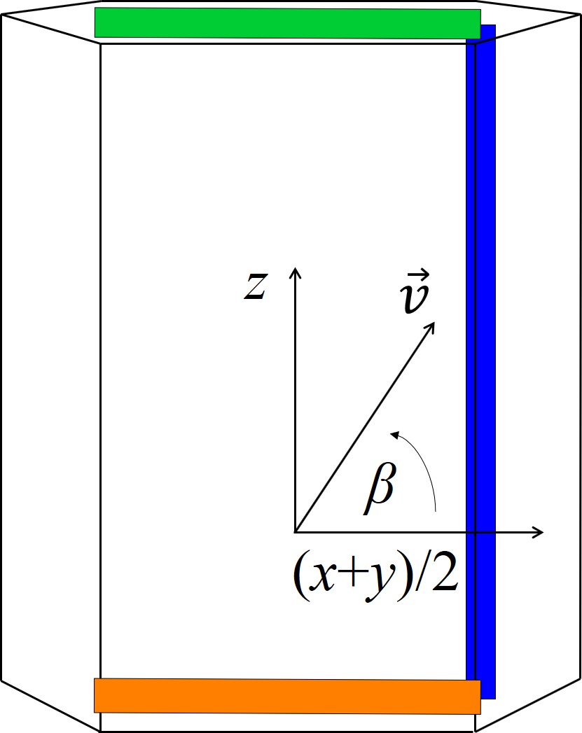
Figure 2.16: Schematic representation of the hexagonal crystal structure in the (a) x-y, (b) x-z, and (c) (x+y)/2-z plane. \(\vec{v}\) is the crystal direction vector, α is an angle in the x-y plane, and β is an angle in the x-z or (x+y)/2-z plane. The blue, red, green, and orange squares represent the a-, m-, Si-, and C-face, respectively.
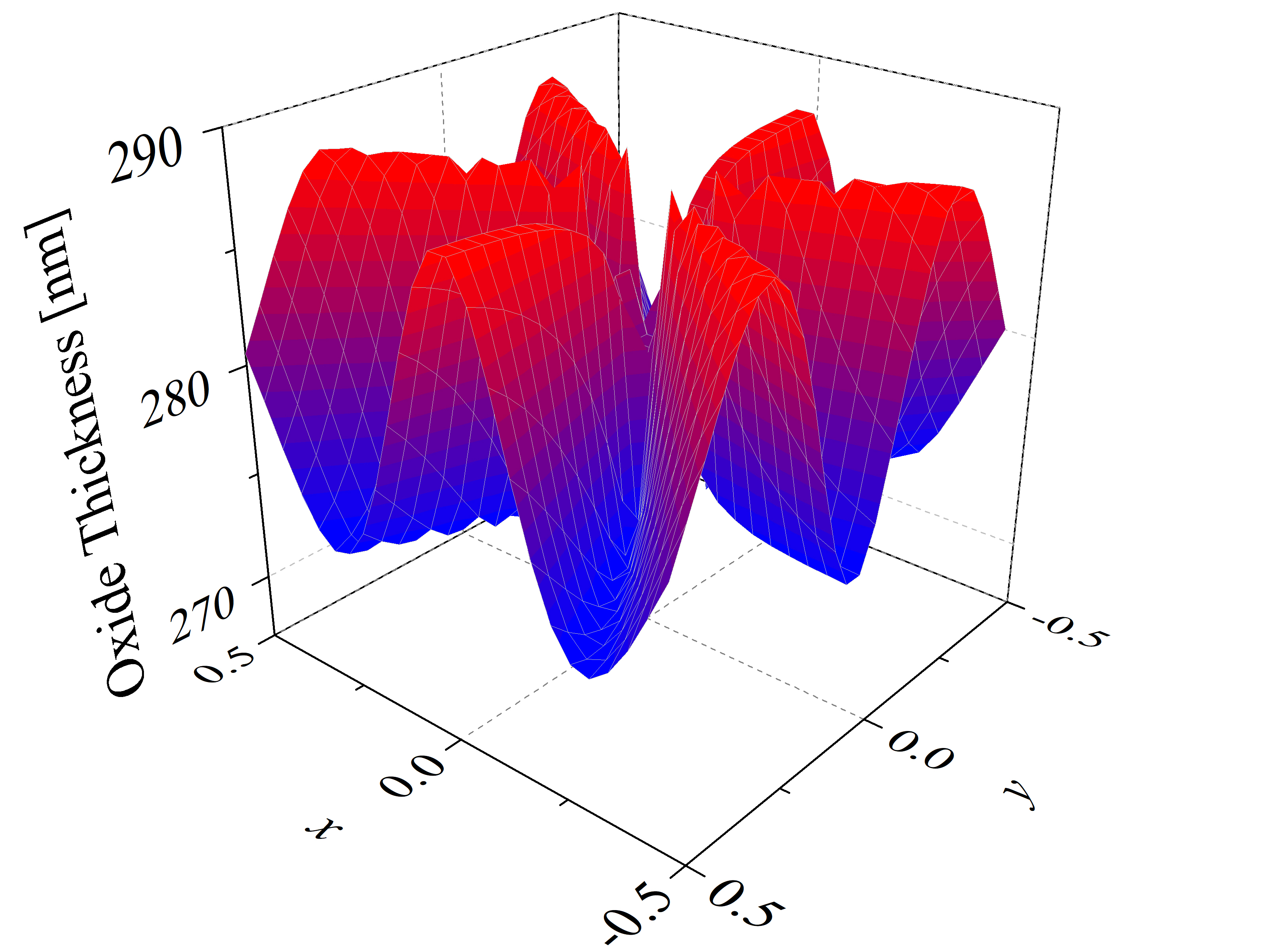
The thicknesses of SiC thermal oxidation in 2D space are calculated with Massoud’s model (cf. Section 2.3.2) and the interpolation method for the growth rate parameters B/A, C, and L. The oxide thicknesses as a function of the vector coordinates x, y, and z (calculated for the x-y and x-z plane) are shown in Figure 2.18. In the first plot six maxima and six minima are observed, which correspond to the m- and a-face, respectively. The final oxide thickness in the direction of the m-face is approximately 288 nm and in the direction of the a-face 273 nm. On the second plot one maximal and one minimal oxide thickness is observed, which correspond to the C- and the Si-face, respectively. The final oxide thickness in the direction of the Si-face is approximately 39 nm and in the direction of the C-face 327 nm. These results are in a good agreement with experimental findings [88].
In order to allow for a straightforward comparison between theoretical calculations and experimental data, the oxide thicknesses X are normalized with the maximal oxide thickness Xmax, such that
\( \seteqsection {2} \) \( \seteqnumber {61} \)
\begin{equation} \hat {X} = X / X_\mathrm {max}. \end{equation}
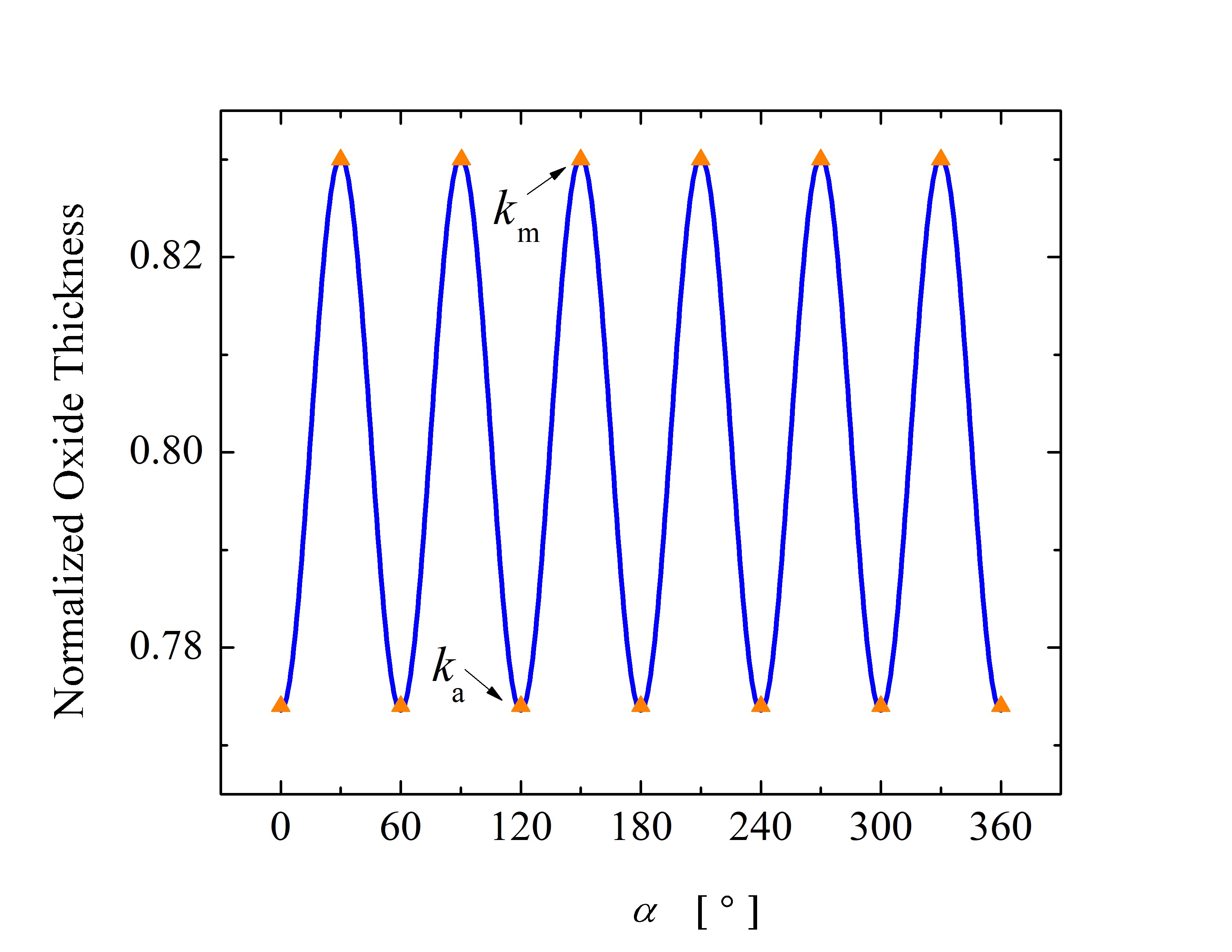
Thus, \(\hat{X}\) = 1 corresponds to the maximum oxide thickness and \(\hat{X}\) = 0 corresponds to no oxide on the surface of SiC. The main goal of such a comparison is to validate and corroborate the ratios between the growth rates for various crystal directions. The oxide thicknesses as a function of α and β, i.e., the angle between the crystal direction vector and the x axis, are shown in Figure 2.19. The calculations are performed for an angle ranging from 0° to 360° for both planes. The calculated results for the normalized oxide thicknesses are in good agreement with available measurements [87].
Moreover, these results provide the basis for multi-dimensional simulations of dry oxidation of 4H-SiC. 2D and 3D simulations can thus be augmented by the interpolation method for the oxidation growth rates, where the only limiting factor is the set of known growth rate values, which is optimally obtained from measurements. The fact that the only limiting factor of the interpolation method is the four extreme growth rates in the Cartesian directions expands the applicability of this approach beyond SiC. It is very likely that the same interpolation method can be utilized for predicting oxidation growth rates for other semiconductor materials, which possess the same hexagonal crystal structure as SiC.
(a)
(b)
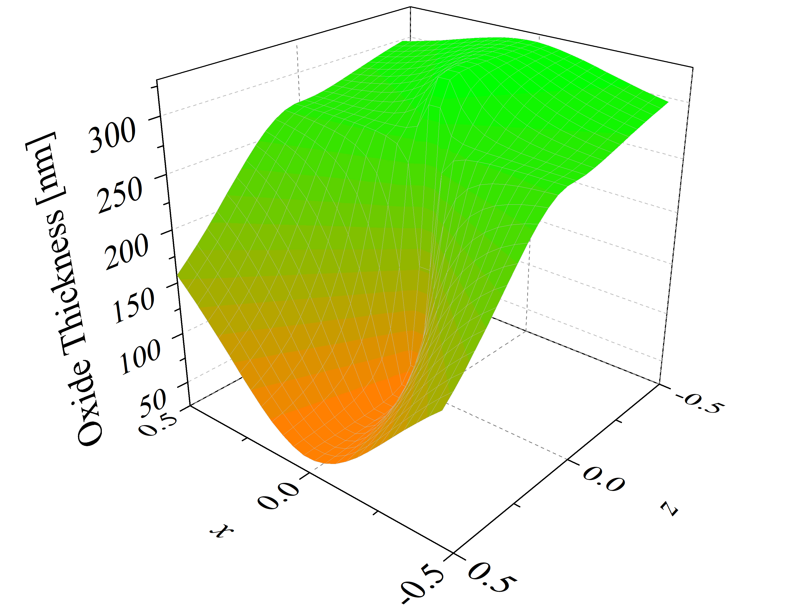
Figure 2.18: 2D calculations of the oxide thicknesses in the (a) x-y and (b) x-z plane. The figures show the final oxide thicknesses as a function of the normalized crystal direction vector coordinates x, y, and z. The red, blue, orange, and green colors represent oxide thicknesses for the m-, a-, C-, and Si-face, respectively. The calculations are performed for oxidation at T = 1100°C for 720 min.
(a)
(b)
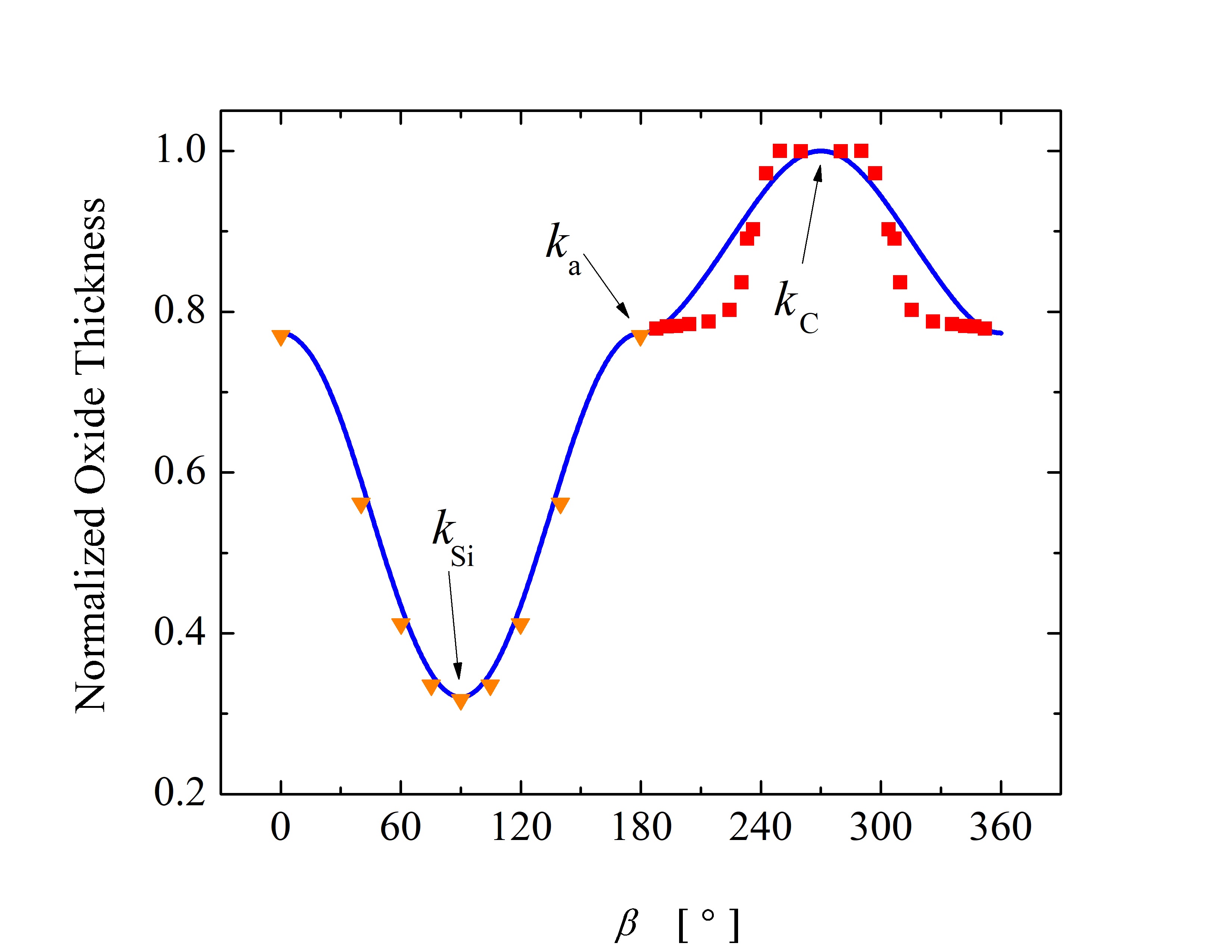
Figure 2.19: Normalized oxide thicknesses as a function of angle (a) α in x-y plane and (b) β in x-z plane as shown in Figure 2.16. The oxide thickness is normalized with the maximal oxide thickness to enable a direct comparison between calculations and experiments. The blue solid lines are calculations performed with Massoud’s model and the presented in- terpolation method. The orange triangles and red squares are measurement results [88, 86]. The black arrows indicate the known growth rates for the interpolation method, i.e., km, ka, kSi, and kC.