in the problem (3.5). The purpose of such a process is to create a controlled sub-space
inside
in the problem (3.5). The purpose of such a process is to create a controlled sub-space
inside  , which can be designed to approximate the solution of (3.6) with arbitrary
precision.
, which can be designed to approximate the solution of (3.6) with arbitrary
precision.
The basics of Galerkin’s method consist of a clever discretization of the infinite linear space
in the problem (3.5). The purpose of such a process is to create a controlled sub-space
inside , which can be designed to approximate the solution of (3.6) with arbitrary
precision.
Consider the finite sub-space  of
of  with dimension N. Consider also the functions
 as an orthogonal basis of
  . Hence, every function
  in
in  can be written as
linear combination of the basis as in
can be written as
linear combination of the basis as in
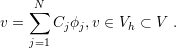 | (3.9) |
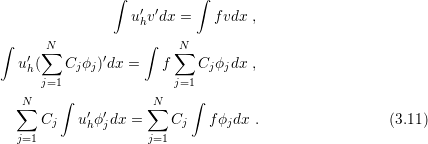
The discrete formulation of the variational problem (3.5) can be written as
 | (3.10) |
Actually, the formulation (3.10) can be simplified. It can be proven that if  satisfies
(3.10) only for the basis function of
satisfies
(3.10) only for the basis function of  , it satisfies it for every element in
  . To show
this, replace
. To show
this, replace  in (3.10) by the basis projection (3.9) as in
On the assumption 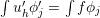 for j = 1..N, the equality (3.11) holds and
  satisfies
(3.10) for every element of
satisfies
(3.10) for every element of  . Consequently, the simplified version of (3.10) can be
summarized by:
. Consequently, the simplified version of (3.10) can be
summarized by:
 | (3.12) |
The formulation (3.12) is well suitable for the construction of a numerical scheme, because it
restricts the search for the solution  to the computation of a finite number of equations
(N). Hence, the problem shifts to a more concrete perspective, and a method
is required to compute
to the computation of a finite number of equations
(N). Hence, the problem shifts to a more concrete perspective, and a method
is required to compute  from those N equations. For that purpose, consider
the expansion of
from those N equations. For that purpose, consider
the expansion of  in the basis of
  , in the same way as was done before
for
, in the same way as was done before
for  (3.9). By substituting
  appropriately in (3.10) the obtained function
is
appropriately in (3.10) the obtained function
is
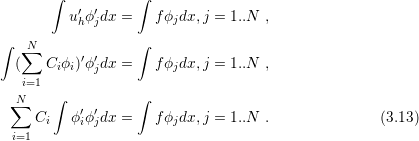
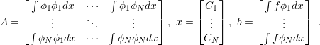
In fact, the substitution of  expansion in (3.12) leads to the transformation of the
discrete problem in a linear system
expansion in (3.12) leads to the transformation of the
discrete problem in a linear system  with N equations, where A, x and b are given
by
with N equations, where A, x and b are given
by
 | (3.14) |