Thermal Expansion

2.2.3 Thermal Expansion

So far the discussion has treated indistinguishably the source of stress. However, for thermal sources a special treatment is suitable, due to its importance in engineering problems. Temperature variation in a solid leads to its expansion or retraction, and consequently to deformations. Thus, thermal strains can be described by

εth = α ΔT ,

(2.23)

where $εth$ is the thermal strain, $ΔT$ is the temperature variation and $α$ is the coefficient of thermal expansion (CTE). Typical values of CTE for materials in semiconductor industry are listed in Table 2.1.

Thermal expansion is an isotropic effect, which means that the material expands according to (2.23) in every direction. Additionally, there is no skew deformations induced by thermal variations, meaning only normal components of the strain tensor are affected. Hooke’s law, with thermal effects included is given by

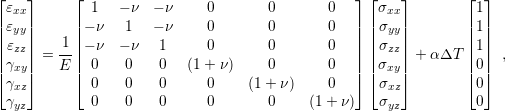⌊εxx⌋ ⌊ 1 − ν − ν 0 0 0 ⌋ ⌊σxx⌋ ⌊ 1⌋ |εyy| |− ν 1 − ν 0 0 0 | |σyy| | 1| ||ε || 1 ||− ν − ν 1 0 0 0 || ||σ || || 1|| || zz|| = --|| || || zz|| + α ΔT || || , |⌈γxy|⌉ E |⌈ 0 0 0 (1+ ν ) 0 0 |⌉ |⌈σxy|⌉ |⌈ 0|⌉ γxz 0 0 0 0 (1 + ν) 0 σxz 0 γyz 0 0 0 0 0 (1 + ν) σyz 0

(2.24)

which can be represented inversely with

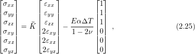
⌊σxx⌋ ⌊ εxx ⌋ ⌊ 1⌋ |σ | | ε | | 1| || yy|| || yy || E αΔT || || |σzz| = K¯¯| εzz | − ------| 1| , (2.25) ||σxy|| || 2εxy|| 1 − 2ν|| 0|| ⌈σxz⌉ ⌈ 2εxz⌉ ⌈ 0⌉ σyz 2εyz 0

where

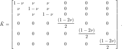⌊ ⌋ 1− ν ν ν 0 0 0 || ν 1− ν ν 0 0 0 || || ν ν 1 − ν 0 0 0 || || (1− 2 ν) || ¯¯K = || 0 0 0 -------- 0 0 || . | 2 (1 − 2ν) | || 0 0 0 0 -------- 0 || |⌈ 2 (1 − 2ν)|⌉ 0 0 0 0 0 -------- 2

To conclude this section, it is worth to make some remarks regarding the presented approach. First, the adopted strain definition is commonly referred as engineering strain, but there are other measures (e.g. True strain [51], Stretch ratio [51], Green strain [40], and Almansi strain [40]) which are particularly useful for describing phenomena outside the infinitesimal strain theory [39][40][41]. Usually, mechanical deformation in semiconductor devices can be properly treated solely by implementing the engineering strain definition, but some scenarios may demand the True strain definition.

Second, Hooke’s law was derived assuming that the solid was made of an isotropic material, which assures that the material constants (E, $ν$ , and $α$ ) are independent of direction. However, for some materials this condition is not valid as in the case of silicon, where the Young modulus can variate between 130GPa and 189GPa depending on the direction [52].

Lastly, in literature it is possible to find Hooke’s law described using other material constants, for example the Lamé parameters [39]. There is a suitable relation between the set of constants and it is a matter of preference or ease of notation for one to use one as opposed to the other.

[next] [prev] [prev-tail] [front] [up]