|
|
|
|
Previous: 4.3.3 Total Scattering Rate Up: 4.3 Zero Field Monte Carlo Algorithm Including the Next: 4.3.5 Monte Carlo Algorithm for the Mobility Tensor |
|
|
|
|
Previous: 4.3.3 Total Scattering Rate Up: 4.3 Zero Field Monte Carlo Algorithm Including the Next: 4.3.5 Monte Carlo Algorithm for the Mobility Tensor |
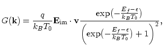 |
(4.50) |
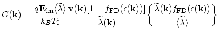 |
(4.51) |
The Monte Carlo algorithm contains the same steps as that in [73] except that the whole kinetics is now determined by
![]() and
and
![]() instead of
instead of
![]() and
and
![]() .
.
Another difference from the non-degenerate zero field algorithm is that the weight coefficient
![]() must be multiplied by the factor
must be multiplied by the factor
![]() .
.
With the modifications described above the zero-field algorithm for the time discrete impulse response of a physical quantity
![]() of
interest becomes:
of
interest becomes:
This algorithm is also depicted in Fig. 4.5.
![\includegraphics[width=0.9\linewidth]{figures/figure_12}](img990.png)
|
S. Smirnov: