4.3.5 Monte Carlo Algorithm for the Mobility Tensor

The response to small signals with a general time dependence can be obtained from the knowledge of the impulse response. The static zero field mobility is given by the long time limit of the differential velocity step response. This is exploited to derive a zero field Monte Carlo algorithm for the mobility tensor from the algorithm presented in the previous section. For a vector-valued physical quantity $\vec{A}$ elements of the differential step response tensor are related to the differential impulse response tensor in the following manner:

$$[K_{A}^\mathrm{step}(t)]_{ij}=\int_{0}^{t}[K_{A}^\mathrm{imp}(t^{'})]_{ij}\,dt^{'},$$ (4.52)

where the differential impulse $[K_{A}^\mathrm{imp}(t^{'})]_{ij}$ and step $[K_{A}^\mathrm{step}(t)]_{ij}$ response tensors are defined through the following relations:

$$\langle A_{i}\rangle_\mathrm{imp}(t)=\sum_{j}[K_{A}^\mathrm{imp}(t)]_{ij}(F_\mathrm{imp})_{j}$$

$$\langle A_{i}\rangle_\mathrm{step}(t)=\sum_{j}[K_{A}^\mathrm{step}(t)]_{ij}(F_{1})_{j}.$$ (4.53)

In order to obtain the zero field mobility tensor it is necessary to integrate the differential velocity impulse response over a secondary trajectory for a sufficiently long time. However, the time integration can be stopped after the first velocity randomizing scattering event has occurred, because in this case the correlation of the trajectory's initial velocity with the after-scattering velocity is lost. 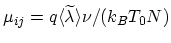Since in the thermodynamic equilibrium the before and after-scattering distributions are equal, the secondary trajectories can be mapped onto the main trajectory. As a result the algorithm schematically depicted in Fig. 4.6 is obtained.

Figure 4.6: Zero field Monte Carlo flow chart.

1. Set $\nu=0$, $w=0$.
2. Select initial state $\vec{k}$ arbitrarily.
3. Compute a sum of weights: $w=w+[1-f_\mathrm{FD}(\epsilon(\vec{k}))][v_{j}(\vec{k})/\widetilde{\lambda}(\vec{k})]$.
4. Select a free-flight time $\widetilde{t}_{f}=-\ln(r)/\widetilde{\lambda}(\vec{k})$ and add time integral to estimator: $\nu=\nu+wv_{i}\widetilde{t}_{f}$ or use the expected value of the time integral: $\nu=\nu+w[v_{i}/\widetilde{\lambda}(\vec{k})]$.
5. Perform scattering. If mechanism was isotropic, reset weight: $w=0$.
6. Continue with step 3 until $N$ $\vec{k}$-points have been generated.
7. Calculate component of zero field mobility tensor as $\mu_{ij}=q\langle\widetilde{\lambda}\rangle\nu/(k_{B}T_{0}N)$.

Especially the diagonal elements can be calculated very efficiently using this algorithm. Consider a system where only isotropic scattering events take place. Then the product $wv_{i}$ is always positive, independent of the sign of $v_{i}$. Therefore, only positive values are added to the estimator, which leads to a low variance.

S. Smirnov: