3. 1. 3 Integration Example

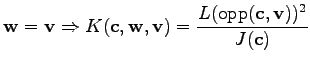
In the implementation of the finite element scheme the actual differential operator is not relevant for algebraic structure of the formalism. This section shows the application of the finite element method to the Laplace equation

$$\Delta u = 0 \; .$$ (3.10)

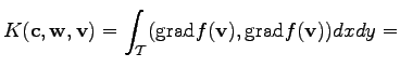
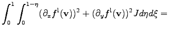
For such an equation functions are required which are twice differentiable. The usual method to reduce this requirement is to apply the Green integral identity where one obtains the following expression

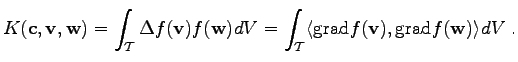$$K (\mathbf{c}, \mathbf{v}, \mathbf{w}) = \int_\mathcal{T} \Delta ... ...angle \mathrm{grad} f(\mathbf{v}) , \mathrm{grad} f(\mathbf{w}) \rangle dV \; .$$ (3.11)

$\mathcal{T}$ denotes the local integration region. Using a geometrical transformation, simplicial elements can be transformed into unity simplices. For other elements, e.g. cuboids, it is also possible to transform the integration domain in order to simplify the calculation. The following considerations concern the standard method of simplicial (triangular) elements and linear shape functions. Methods in which the integrals can be solved analytically can be treated in the same manner.

In most cases the quadrature can be performed analytically, which implies that most of the calculations are carried out before the simulation is started. During the simulation process predetermined numbers are inserted. In many cases, e.g. more complicated differential equations, irregular shapes of the elements, or when using higher order polynomial approaches, it might be of favor to use alternative quadrature methods, mostly numerical quadrature means. In such a case the evaluation of the function $K$ invokes e.g. a Gauß quadrature method. Moreover, it can be stated that a quadrature method for the determination of the integral function $K$ does only require information which is associated with one of the arguments passed. In some special cases it might be desirable to use incidence traversal methods, e.g., to determine values which are associated to edges of the respective cell.

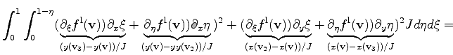
In the following considerations the integrals are not evaluated as a complete matrix but separately for each two vertices on a given triangular cell. The integral is evaluated using the typical geometrical transformation to a standard triangular element with corner points in $(0, 0)$ , $(1, 0)$ and $(0, 1)$ . The local coordinates of the transformation are denoted as $\eta$ and $\xi$ . The associated shape function for the single vertices are $\eta$ , $\xi$ and $1 - \eta - \xi$ . A transformation function can be found in the following way:

$$x = \xi (x_2 - x_1) + \eta (x_3 - x_1)$$ (3.12)

$$y = \xi (y_2 - y_1) + \eta (y_3 - y_1) \; ,$$ (3.13)

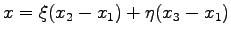
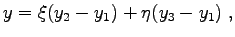
where $x_n$ and $y_n$ denote the vertices of the triangle in any ordering. The derivatives of the variables in the standard range $\eta, \xi$ with respect to the original variables $x, y$ are:

$$\partial_x \xi = \frac{y_3 - y_1}{J}, \qquad \partial_y \xi = \fr... ...x \eta = \frac{x_3 - x_1}{J}, \qquad \partial_y \eta = \frac{x_2 - x_1}{J} \; .$$ (3.14)

Here, $J$ denotes the determinant of the transformation matrix. Together with this determinant the differentials can be transformed. The determinant is defined with respect to the cell. For the calculation the coordinate values of the vertices are required.

$$J = (x_2 - x_1)(y_3 - x_1) - (x_3 - x_1)(y_2 - y_1), \qquad dx dy = J d\eta d\xi \; .$$ (3.15)

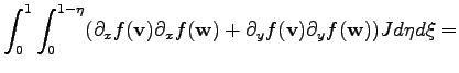
In the first case of the evaluation of the function $K$ , the vertices $\mathbf{w}$ and $\mathbf{v}$ coincide and the point $(0, 0)$ is used as point of the common vertex. The common shape function is denoted as $f(\mathbf{v}) = f(\mathbf{w}) = f(\mathrm{c}) = 1 - \xi - \eta$ .

$$K (\mathbf{c}, \mathbf{w}, \mathbf{v}) = \int_\mathcal{T} ( \mathrm{grad} f(\mathbf{v}), \mathrm{grad} f(\mathbf{v})) dx dy =$$

$$\int_0^1 \int_0^{1-\eta} (\partial_x f^{\mathrm{l}}(\mathbf{v})) ^ 2 + (\partial_y f^{\mathrm{l}}(\mathbf{v})) ^ 2 J d\eta d\xi =$$

$$\int_0^1 \int_0^{1-\eta} ( \underbrace{\partial_\xi f^{\mathrm{l}... ...f{v})) \partial_y \eta}_{(x(\mathbf{v})-x(\mathbf{v}_3))/J}) ^ 2 J d\eta d\xi =$$

$$\int_0^1 \int_0^{1-\eta} (y_3-y_2)^2 + (x_3-x_2)^2 / J d\eta d\xi... ...hbf{v}_2)\Vert}{2 J} = \frac{l(\mathrm{edge}(\mathbf{v}_3, \mathbf{v}_2))}{2 J}$$ (3.16)

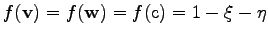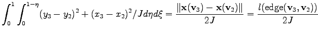
It can be seen that the value of the integral depends on the volume of the cell as well as on the length of the edge opposing the common edge (see Fig. 3.3). For this reason a topological function $\mathrm{opp}(\mathbf{c}, \mathbf{v})$ can be introduced which returns the edge opposing a vertex within a triangular cell. The quantities $J$ and $L$ are defined on the cells and edges, respectively.

Figure 3.3: The opposing edge of a vertex within a cell.

$$\mathbf{w} = \mathbf{v} \Rightarrow K (\mathbf{c}, \mathbf{w}, \mathbf{v}) = \frac{L(\mathrm{opp}(\mathbf{c}, \mathbf{v}))^2}{J(\mathbf{c})}$$ (3.17)

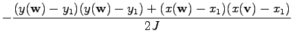
For the second case it is assumed that the vertices $\mathbf{v}$ and $\mathbf{w}$ are different. In this case, the vertices $\mathbf{v}$ and $\mathbf{w}$ are located on the points $(1, 0)$ and $(0, 1)$ . The shape function collocated with $\mathbf{v}$ is referred to as $f(\mathbf{v})$ and the shape function collocated with $\mathbf{w}$ is referred to as $f(\mathbf{w})$ .

$$\mathbf{w} \neq V \Rightarrow K (\mathbf{c}, \mathbf{w}, \mathbf{v}) =$$

$$\int_\mathcal{T} ( \mathrm{grad} f(\mathbf{v}), \mathrm{grad} f(\mathbf{w}) ) dx dy =$$

$$\int_0^1 \int_0^{1-\eta} (\partial_x f(\mathbf{v}) \partial_x f(\mathbf{w}) + \partial_y f(\mathbf{v}) \partial_y f(\mathbf{w})) J d\eta d\xi =$$

$$-\frac{(y(\mathbf{w})-y_1)(y(\mathbf{w})-y_1) + (x(\mathbf{w})-x_1)(x(\mathbf{v})-x_1)}{2 J}$$ (3.18)

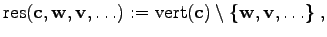
To precisely specify this formula using the formalism presented in Chapter 2, the localities of the quantities are defined exactly, for the third vertex within the triangular cell, the following topological function can be used (see Fig. 3.4).

$$\mathrm{res}(\mathbf{c}, \mathbf{w}, \mathbf{v}, \ldots ) := \mathrm{vert}(\mathbf{c}) \setminus \{\mathbf{w}, \mathbf{v}, \ldots\} \; ,$$ (3.19)

Figure 3.4: The third vertex within a triangle. $\mathbf{x} = \mathrm{res}(\mathbf{c}, \mathbf{v}, \mathbf{w})$ .

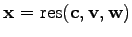where the function $\mathrm{vert()}$ denotes all vertices incident with a cell. The final formula yields

$$K (\mathbf{c}, \mathbf{v}, \mathbf{w}) = [ \bigwedge_{\underline{... ...\underline{z}})} {2 J_{\underline{1}}} ] ] (\mathbf{c}, \mathbf{v}, \mathbf{w})$$ (3.20)

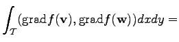
These considerations can be performed for other differential operations, element shapes, and shape functions, as long as the integrals are evaluable analytically. As the necessary quantities and geometrical properties are always associated with topological elements incident to the common cell, further topological functions such as the opp() function may become relevant for the calculations. One restriction which is crucial for the evaluation of the integral term $K$ is that only quantities are required which are associated with elements that are incident with the cell $C$ or which are global.