Electronic products introduced to the market have to fulfill specific quality criteria. There are definitely major differences in the customer's expectations depending on the product type and application field. It appears commonly acceptable if a cheap give-away gadget fails after one year. On the other hand, malfunctioning of an airbag system in a ten year old car is a serious, safety relevant failure. This shows that the customers expectations on the reliability depend on the product. Especially high expectations are associated with safety and security components.
The IEEE defines reliability as the ability of an item to perform a required function under stated conditions for a stated period of time [7]. In this context, an item can be any system or product, e.g. a mobile phone, an integrated power amplifier, or an airbag system. For the discussion on reliability a specification that defines good and failed devices is required. Specifications have to include tolerances, therefore, a changing device parameter does not automatically imply a failure. They also have to include the allowed operating conditions, including circuitry and environmental impacts. Note that the IEEE definition also includes the factor time, highlighting its importance when talking about reliable or unreliable components. However, not only the operating time but also the storage time for devices on stock has to be considered. This is on one hand important for components which are not permanently used and wearout therefore cannot be monitored, and, on the other hand, for articles that are kept on stock for long periods. This is especially the case for spare parts.
Beginning from the early stages of the industrialization of electricity, reliability was and still is a major concern. It is also often a show-stopper for the introduction of new technologies. Looking back in history, it required nearly 70 years until the reliability of the incandescent light bulb was high enough to make electrical lighting commercially interesting. Engineers had put much effort into finding materials used for the filament as well as for the gas surrounding it. Further technological advances finally offered high-performance vacuum pumps. This made the fabrication of the evacuated bulbs possible, which finally became even more successful. This example shows that reliability is important for new products and that the two key issues for the development of reliable products are materials and technology.
One of the first systematic approaches for investigating system reliability and reliability prediction was initiated by military institutions. The topic became important due to the high failure rates of electronic equipment during World War II. The common approach to keep systems in operation was to stock up spare parts. However, this logistically challenging and very cost intensive. Hence, the demand emerged to increase and to quantitatively specify the reliability. In 1952 the U.S. Defense Department founded together with electronics industry the Advisory Group on Reliability of Electronic Equipment (AGREE) whose charter was to identify actions that could be taken to provide more reliable electronic equipment [56]. Soon after, the reliability community split into supporters of two general approaches [57]. On one side there is a community supporting the physics-of-failure models which could be described as bottom-up approaches [58]. On the other side, there are the proponents of empirical models which are solely based on historical data. In this context, historical data means collected information from comparable systems previously designed, manufactured, and already used. Only for those system is historical data like wearout and lifetime available. This empirical approach originates from the desire to determine the prospective reliability of systems from the beginning of the design phase long before specific parts have been selected. This strategy can be considered as top-down approach. One of the oldest and for a long time widely accepted document giving guidelines on reliability estimations using empirical based models is the MIL-HDBK-217 [59] entitled ``Reliability Prediction of Electronic Equipment''. The first release was issued in 1962 by the US Department of Defense. Even if this document was widely used, many authors criticized the proposed failure-rate prediction. The obvious problem of a design guideline that is based on historical data is the delay between the introduction of new materials and technologies and the availability of collected field data. This prevented the use of benefits of new developments for a long time [60]. Furthermore, engineers emphasized the important missing links between stress history, environmental impacts, and actual cause of failure.
In contrast to empirical methods, physics-of-failure approaches have the goal to identify the root failure mechanism based on physical principles [61]. This approach helps to localize the problem and to improve components efficiently. Criticism of this approach concerns the increased complexity using physics-based modeling and the incapability of this low-level approach to capture a complex system as a whole. For a long time proponents of empirical and physics-of-failure approaches were arguing with each other, which method is better and should be used. Morris et al. [62] concluded that both methods have their according application field and should be used in conjunction. However, the reliability investigations in this work only consider physical impacts on the device and therefore only contribute to the physics-of-failure approach.
Systems are often required to be available and working for a certain amount of time during their lifetime. Manufactures or service operators have to guarantee their customers that a given device or infrastructure operates at least for a specific time per month/year. This implies that the system can be repaired and maintainability is given. Failed systems can therefore be restored to working condition by repairing or changing parts. However, for a single semiconductor device, maintainability is not given, since failures cannot be repaired. Hence, in reliability engineering the term survivability is used for systems that cannot be repaired. This is also used when a repair is not an option. This is true for cheap products, e.g. inkjet printing cartridges, or for products where once set in operation, repair is impossible, for example, due to inaccessibility.
Considering a specific physical failure, one has to distinguish between failure mode and failure mechanism or failure cause. A symptom observed in a failed or degraded device is called failure mode. This can be, for example, an increased current or an open circuit. A failure mode can be caused by different physical failures, so-called failure mechanisms. The same failure mechanism does not necessarily lead to the same failure mode. An oxide breakdown, for example, can lead to a short or to an open circuit. The open circuit can also be caused by some other failure mechanism, for example by electromigration.
The statistical temporal distribution of failures can be visualized using the hazard curve. This curve shows the devices failure rate, also known as hazard rate, over the operating time. The widely accepted typical shape of the hazard curve is the bathtub curve shown in Fig. 3.1. This curve is originally derived from the life expectations of humans.
![\includegraphics[width=0.49\textwidth]{figures/hazard_bathtub}](img79.png)
|
In this theory, the lifetime of a system is split into three major parts. In the first part a high failure rate can be observed, called the infant mortality. This is reasoned to be due to major weaknesses in materials, production defects, faulty design, omitted inspections, and mishandling [63]. These failures are also considered as extrinsic failures [64] and it is suggested that all systems with gross defects fail during the early operation time. This leads to the next period, the system's useful time. Here, a low failure rate can be observed. This part is often modeled using a constant failure rate. Therefore, the probability of a system to fail is randomly distributed. Even though this assumption is heavily debated, many reliability calculations are based on such a constant rate. At the end of the lifetime, the wearout period follows due to fatigue of materials. An intelligent product design makes sure that wearout occurs after some time greater than the planned lifetime of the product [64].
One of the strong opponents of the bathtub curve is Wong [65,66,67] who suggested that the hazard rate follows a roller-coaster curve as shown in Fig. 3.2.
![\includegraphics[width=0.49\textwidth]{figures/hazard_rollercoaster}](img80.png)
|
He initiated the idea, that the constant failure rate throughout the useful life is not caused by randomly distributed errors. Instead, weaknesses in sub-items of the whole electronic system cause one or more humps. He assumes, that these are extrinsic failures already present but not found after fabrication. Wong stated that the constant failure rate has been defended for so long because it is based on tainted field data. On the other hand, the failure rate in the useful lifetime can be attributed partly to environmental impacts which are not intrinsic to the device. The occurrence of those external events, like an electrostatic discharge event, are furthermore random and, therefore, lead to a nearly flat phase in the hazard curve. If these external events are included in the total reliability of the electronic system, the bathtub curve becomes valid again.
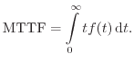
Traditional reliability calculations are based on statistical data collected
using failure records. For ![]() statistically identical and independent items
the time between putting the device into service and occurrence of a failure
can be collected. This can be used to determine the empirical expectation value
for the mean failure-free time
statistically identical and independent items
the time between putting the device into service and occurrence of a failure
can be collected. This can be used to determine the empirical expectation value
for the mean failure-free time ![]() as
as
| (3.1) |
| (3.3) |
 |
(3.5) |
 |
(3.6) |
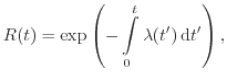
Different failure distributions ![]() have been used to describe the failure
events for devices and systems. A convenient modeling approach is to apply a constant failure rate. This is
also assumed for the useful time phase in the bathtub curve. The guidelines in
MIL-HDBK-217, too, are based on this approach. Using
have been used to describe the failure
events for devices and systems. A convenient modeling approach is to apply a constant failure rate. This is
also assumed for the useful time phase in the bathtub curve. The guidelines in
MIL-HDBK-217, too, are based on this approach. Using
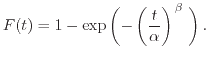
![]() yields an exponential distribution. The probability density function results in
yields an exponential distribution. The probability density function results in
![\includegraphics[width=0.49\textwidth]{figures/exp_DF}](img99.png)
![\includegraphics[width=0.49\textwidth]{figures/exp_CDF}](img100.png)
![\includegraphics[width=0.49\textwidth]{figures/exp_HF}](img101.png)
|
The probability that a failure event occurs is equal for any point in time, no
matter how old the device is. This means that a device that as an age ![]() is as
good as a new item [68]. This characteristic is called memoryless and
makes calculations possible without knowledge of the past operating time. In
the first reliability models, it was assumed that the failure rate is constant
over the device lifetime. However, this seems not to be the case, as already
explained in the context of the bathtub curve. It is suspected that the
constant failure rate was assumed due to systematic errors and
misinterpretation of results during data acquisition [63]. For
example, due to continuous repair work performed on the test system, in fact
data of time-in-between-failures, which has a constant failure rate, was mixed
with data of time-to-failure measurements.
is as
good as a new item [68]. This characteristic is called memoryless and
makes calculations possible without knowledge of the past operating time. In
the first reliability models, it was assumed that the failure rate is constant
over the device lifetime. However, this seems not to be the case, as already
explained in the context of the bathtub curve. It is suspected that the
constant failure rate was assumed due to systematic errors and
misinterpretation of results during data acquisition [63]. For
example, due to continuous repair work performed on the test system, in fact
data of time-in-between-failures, which has a constant failure rate, was mixed
with data of time-to-failure measurements.
For the description of more realistic failure rates numerous other distribution functions have been used. Two prominent examples are the Weibull and the lognormal distribution. The latter one is derived from the normal distribution by taking natural logarithms of all data points. The probability density function is given by
 |
(3.10) | |
 |
(3.11) |
![\includegraphics[width=0.49\textwidth]{figures/lognorm_DF}](img110.png)
![\includegraphics[width=0.49\textwidth]{figures/lognorm_CDF}](img111.png)
![\includegraphics[width=0.49\textwidth]{figures/lognorm_HF}](img112.png)
![\includegraphics[width=0.49\textwidth]{figures/Ohring_Lognormal.eps}](img113.png)
|
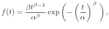
The Weibull distribution, shown in Fig. 3.5 can be used to model monotonous falling or rising hazard curves.
![\includegraphics[width=0.49\textwidth]{figures/weibull_DF}](img114.png)
![\includegraphics[width=0.49\textwidth]{figures/weibull_CDF}](img115.png)
![\includegraphics[width=0.49\textwidth]{figures/weibull_HF}](img116.png)
![\includegraphics[width=0.49\textwidth]{figures/Weibull_Oxide}](img117.png)
|
The density function for the Weibull distribution reads
Statistical reliability considerations help to quantify the expected lifetime of electronic components and systems. Distribution functions are used to describe the expected failure rate of a certain population but it is not possible to make a prediction for a certain device. There is only a weak link between this statistical modeling approach and the underlying physics. Very often, this link is missing at all. To improve the reliability and to make more physics-based predictions, it is required to take a closer look at the failure mechanisms and the underlying physics. Using this insight also helps to improve the reliability as well as reliability predictions.
To run a semiconductor production line economically, one of the most important key figures is to reach high yield. Yield describes the number of useful devices at the end of the production line in relation to the number of potentially useful devices at the beginning of processing [74]. Therefore, all defects which can be detected after manufacturing are called yield defects. Hence, yield can also be described as the probability that a device has no yield defects [75].
Defects introduced during production which are not detected, can lead to device failures. This failure type can be classified as extrinsic failure. This gives a relation between reliability and yield. Huston et al. [64] have shown this correlation by considering the size of defects introduced during processing. In his work, the defect size on interconnects was investigated, but the model was also applied for gate oxide yield [76,75], where defects are considered as a local effective oxide thinning [77].
In these considerations, large defects resulting in non-working devices are detected in the production line or during device tests. These defects are therefore called yield defects and the devices are rejected [64]. The smallest failures might have negligible effects or might lead to random reliability failures during the lifetime of the device. In between are intermediate sized defects which might be detected during fabrication but might also remain undiscovered. Hence, these defects especially tend to cause infant mortality. Usually burn-in tests are used to prevent that those devices are delivered to customers. Note, that the distinction between large and small defects depend on the defect type and is obviously different for the two oxides and interconnects
![\includegraphics[width=0.6\textwidth]{figures/defect_size}](img122.png)
|
A defect size distribution, as schematically shown in Fig. 3.6, allows to estimate correlations between reliability and yield. Various investigations on this relation have confirmed this by using field data from different fabrication lines and different processes [64,78]. Devices coming from batches which reached high yield show a lower infant failure rate. This can be explained by the overall lower failure rate which also reduces the number of reliability failures appearing in the form of extrinsic failures. Since ongoing productions are monitored and optimized, mature processes commonly have higher yield. At the same time, the reliability is also increased.
![$\displaystyle f(t) = \frac{1}{\sigma t \sqrt{2 \pi}} \exp \left[ - \frac{1}{2 \sigma ^2} \left( \ln \left( \frac{t}{\mu} \right) \right)^2 \right] ,$](img102.png)