There are different methods of how directed quantities can be represented in
box discretized systems. In the initial divergence equation
(7.1) the vector quantities
![]() is transformed into
one-dimensional edge discretized values
is transformed into
one-dimensional edge discretized values ![]() which are subsequently used to
assemble the box and flux equations. The single fluxes are estimated using
quantities defined at the end nodes of the edges, like in relation
(7.6) for the dielectric flux and (7.7) for the
current density. No vector quantities are required to assemble the basic
equations. However, vector attributes like the electric field and the current
density are needed for the calculation of physical models. The electric field
and the current density are required, for example, to model the high-field
mobility or the impact-ionization rate in the drift-diffusion framework. For the representation of
attributes as vector quantity, additional methods are required, some are
represented in this section.
which are subsequently used to
assemble the box and flux equations. The single fluxes are estimated using
quantities defined at the end nodes of the edges, like in relation
(7.6) for the dielectric flux and (7.7) for the
current density. No vector quantities are required to assemble the basic
equations. However, vector attributes like the electric field and the current
density are needed for the calculation of physical models. The electric field
and the current density are required, for example, to model the high-field
mobility or the impact-ionization rate in the drift-diffusion framework. For the representation of
attributes as vector quantity, additional methods are required, some are
represented in this section.
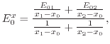
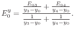
In the work of Laux et al. [263] a discretization scheme is introduced for
the accurate evaluation of the impact-ionization rate. The model assumes an unstructured
triangular mesh. Since the potential and the electric field are based on linear
functions, an electric field vector can be evaluated in a straightforward
manner, consistent with the Poisson discretization. In a triangle ![]() each
pairwise linear combination of
each
pairwise linear combination of
![]()
![]() and
and
![]() gives the same constant value for the electric field
gives the same constant value for the electric field
![]()
Due to the non-linear dependence of the current density
![]() on the carrier
concentrations in the Scharfetter-Gummel discretization, each linear
combination of
on the carrier
concentrations in the Scharfetter-Gummel discretization, each linear
combination of
![]()
![]() and
and
![]() gives a
different current density vector
gives a
different current density vector
![]() The system in the triangle is
overdetermined. Laux suggested to partition each triangle into three avalanche
regions associated with each edge as shown in Fig. 7.8.
The system in the triangle is
overdetermined. Laux suggested to partition each triangle into three avalanche
regions associated with each edge as shown in Fig. 7.8.
![\includegraphics[width=0.36\textwidth]{figures/laux_tri.eps}](img687.png) |
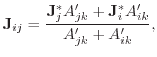
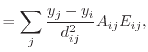
In this work, a current vector is defined for each avalanche region, i.e. for
each edge. Note, that in the notations used here, the indices for the carrier
type specification have been omitted. The current
![]() associated to the
edge between the vertices
associated to the
edge between the vertices ![]() and
and ![]() for example, is defined as
for example, is defined as
 |
(7.13) |
 |
(7.14) |
This approach for vector discretization gives good results as discussed in Section 7.3.3. The limitation to triangular grids (although an extension to tetrahedra is possible) and the higher complexity during equation assembly seem to be the main disadvantages of this method compared the box based vector discretization schemes presented in the next section.
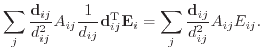
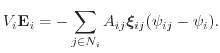
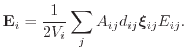
Considering the calculation of the summand in the box approach (7.10), it seems to be most convenient to estimate the vectorial attribute for each box volume, i.e. for each vertex. The model evaluation within the box can then be performed straightforwardly, since all quantities, scalar and vectorial, are then available for the whole box. The results of model evaluation can be directly applied to the box integration equation. In the following, two schemes of vector discretization within boxes are presented. In addition to the simple coupling to the box discretization method, both approaches give accurate approximations for homogenous fields and are numerically stable.
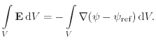
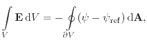
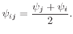
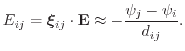
The first scheme follows the derivation of the box discretization scheme itself [271]. Similar to the discussion regarding the right hand side of the box integral, the discretized vector quantities are assumed constant over the whole Voronoi box volume. The derivation of an according discretization scheme is shown for the electric field and can be generalized to auxiliary gradient fields. The electric field is defined as
| (7.15) |
 |
(7.16) |
 |
(7.17) |
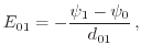
The discretization scheme is also analyzed in a one-dimensional formulation
applying a linearly changing electric field
![]() and an
corresponding quadratic electrostatic potential
and an
corresponding quadratic electrostatic potential
![]() Using
only the x-axis and the naming convention from Fig. 7.9,
(7.21) can be reduced for the linearly changing field to
Using
only the x-axis and the naming convention from Fig. 7.9,
(7.21) can be reduced for the linearly changing field to
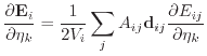
The second discretization scheme is an extension of the finite difference
method and is based on a scheme suggested by Fischer [272]. The
evaluation concentrates on the vector at the vertex itself. Considering the box
0 in a non-equidistant orthogonal mesh depicted in Fig. 7.9 and
its neighboring box 1 (not shown explicitly), the electric field along the
edge ![]() can be expressed as
can be expressed as
![]()
![\includegraphics[width=0.45\textwidth]{figures/box.eps}](img719.png) |
At the boundary between the two boxes, i.e. the midpoint between 0 and 1, the finite difference method gives
 |
(7.24) |
 |
(7.28) |
 |
 |
(7.29) |
 |
 |
(7.30) |
 |
 |
(7.31) |
 |
 |
(7.32) |
 |
(7.33) |
Note that (7.25) and (7.26) are still
retained and can be extracted by using
![]() and
and
![]() respectively.
respectively.
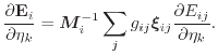
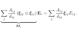
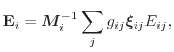
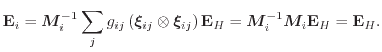
![]() at the left side of
(7.34) can be taken out of the sum and the remaining part of the sum
results in a pure geometry dependent matrix, which is calculated once in the
beginning of the simulation. This allows the convenient formulation of the
final discretization rule for a vector
at the left side of
(7.34) can be taken out of the sum and the remaining part of the sum
results in a pure geometry dependent matrix, which is calculated once in the
beginning of the simulation. This allows the convenient formulation of the
final discretization rule for a vector
![]() in point
in point ![]() as
as
Similar to Scheme A, the validation for homogenous fields using
![]() and
the electrostatic potential
and
the electrostatic potential
![]() is shown. Again, the
relations
is shown. Again, the
relations
![]() and
and
![]() are inserted into
(7.35) which leads to
are inserted into
(7.35) which leads to
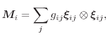
The geometry matrix
![]() introduced in this discretization scheme needs to be
inverted for evaluation. The matrix results from a sum of symmetric matrices
introduced in this discretization scheme needs to be
inverted for evaluation. The matrix results from a sum of symmetric matrices
![]() whose determinants equal to 0
and whose main
diagonals are positive. The sum of matrices with these constraints and with
non-negative determinants also result in a symmetric matrix with positive main
diagonal and a non-negative determinant. If at least two of the participating
matrices are linearly independent, the determinant of the geometry matrix is
positive which is the case as long as the Delaunay criterion is fulfilled. The
inverse of the geometry matrix can therefore always be calculated.
whose determinants equal to 0
and whose main
diagonals are positive. The sum of matrices with these constraints and with
non-negative determinants also result in a symmetric matrix with positive main
diagonal and a non-negative determinant. If at least two of the participating
matrices are linearly independent, the determinant of the geometry matrix is
positive which is the case as long as the Delaunay criterion is fulfilled. The
inverse of the geometry matrix can therefore always be calculated.
 |
(7.40) |
 |
(7.41) |
In this comparison, the vector discretization scheme proposed by Laux and the two box discretized schemes where implemented in MINIMOS-NT and used to calculate the impact-ionization rate. The generation integral on the right hand side of the continuity equation is assembled using (7.10) and (7.12), respectively. The implementation of the scheme by Laux is only limited to two-dimensional domains using triangular meshes, whereas the two other schemes are dimension and mesh independent and the same program code can be used for two- and three-dimensional simulations.
Simulation results from two devices are presented. The first device is a diode
which was selected to investigate effects in a simple one-dimensional
device. The second device used for the comparison is a parasitic
n![]() -p-n-n
-p-n-n![]() structure of a smart power
device which is significantly influenced by the two-dimensional extension. The
diode uses an equidistant mesh and is investigated in reverse-biased operating
condition for different mesh spacings. The parasitic bipolar smart power
structure is simulated in snap-back, a state the device can be driven in during
voltage peaks on the power line.
structure of a smart power
device which is significantly influenced by the two-dimensional extension. The
diode uses an equidistant mesh and is investigated in reverse-biased operating
condition for different mesh spacings. The parasitic bipolar smart power
structure is simulated in snap-back, a state the device can be driven in during
voltage peaks on the power line.
Simulations on the diode structure clearly show that the mesh dependency is higher for the two box based discretization schemes. Using a high mesh density results, as expected, in a comparable output for all three discretization methods. Using a coarser mesh spacing, the results using Laux's scheme change very little, whereas the two box based schemes show larger deviations. In Fig. 7.10 an example using the diode clearly shows that an increased mesh spacing leads to a shift of the breakdown voltage using the box based schemes, whereas only a very small shift is observed using the scheme by Laux.
|
The results for the snap-back simulation in the smart power device are depicted in Fig. 7.11 and show only small deviations between the three schemes. The two box based schemes again show a voltage shift in comparison to the scheme by Laux. The latter one fits well to the reference solution which was generated using a high mesh density (not shown in the figure). The reason for the stronger mesh dependence of the box based schemes can be found in the implicitly finer discretization used in Laux's scheme.
|
The influence of the vector discretization scheme on the convergence behavior is also investigated on the reduced smart power structure as shown in Fig. 7.11(b). Only very little differences were noted and no trend favoring one or another scheme was observed. The convergence process is tracked using the norm of the right hand side. The investigated simulation step is a numerically critical current level step at the triggering phase of the snap-back. It can be clearly seen that the choice of discretization method has only very little influence, despite the critical simulation step.
Although the Laux scheme gives results with a higher accuracy, the influence on the convergence behavior seems to be negligible. On the other hand, the box based schemes can be coupled straightforwardly to the box discretization scheme. Additionally, it is possible to reuse the same implemented code for arbitrary meshes in all dimensions. Throughout this work, the box based Scheme B has been used for all drift-diffusion simulations.
![$\displaystyle \ensuremath{\mathbf{E}}_i = \frac{1}{2V_i} \left[ \sum_j \ensurem...
...}}_{ij} \right) \right] \ensuremath{\mathbf{E}}_H = \ensuremath{\mathbf{E}}_H .$](img712.png)

![\includegraphics[width=0.51\textwidth]{figures/discr_diode.eps}](img767.png)
![\includegraphics[width=0.51\textwidth]{figures/discr_diode_error.eps}](img768.png)
![\includegraphics[width=0.51\textwidth]{figures/error2.eps}](img769.png)
![\includegraphics[width=0.51\textwidth]{figures/convergence.eps}](img770.png)