Subsections

• 4.1 The Model
• 4.2 The Quantum Correction Model
• 4.3 Comparison with Device-SMC
  • 4.3.1 Long Channel Device
  • 4.3.2 Short Channel Devices
  
  
• 4.4 SRS in Macrsocopic Models
• 4.5 Subband versus Bulk

4. Subband Macroscopic Models

IN ORDER TO ACCURATELY describe carrier transport in the inversion layer of a whole device, a 2D non-parabolic macroscopic transport model up to the sixth order has been developed. To include inversion layer effects and to characterize high field transport, a special transport parameter extraction technique from SMC simulations has been carried out. Surface-roughness scattering as well as quantization are thus inherently considered in the SMC tables as described in the previous chapter. Now it is possible to specify higher-order mobilities as well as the macroscopic relaxation times as a function of the effective field. To verify the validity of the 2D macroscopic models, the results are benchmarked against device-SMC simulations. The models are applied to UTB SOI MOSFETs and their predictions are discussed for different channel lengths.

4.1 The Model

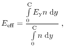
As shown in Fig. 4.1, the extracted higher-order transport parameters derived from SMC forms the base for a parameter interpolation within the channel of the device simulator. In the source and in the drain region the transport parameters are set as constant. The device simulator calculates the transverse effective field in the channel, which is the field perpendicular to the current flow defined as

$$\ensuremath{E}_{\mathrm{eff}}=\frac{\ensuremath{\int\limits_{0}^{... ...h{\int\limits_{0}^{\mathrm{C}}\ensuremath{n}\ensuremath{{\;}\mathrm{d}}y}}{\;},$$ (4.1)

and extracts from the SMC tables the mobilities and relaxation times as a function of the effective field. The upper integration limit $\mathrm{C}$ of equation (4.1) is the channel thickness. The calculated effective field in Fig. 4.2 for different drain voltages $\mathrm{V}_{\mathrm{d}}$ of ${\mathrm{0.1}}{\;}{\mathrm{V}}$ , ${\mathrm{0.25}}{\;}{\mathrm{V}}$ , and ${\mathrm{0.5}}{\;}{\mathrm{V}}$ throughout a ${\mathrm{40}}{\;}{\mathrm{nm}}$ channel length SOI MOSFET device are shown, while the extracted higher-order parameter-set from SMC simulations for different effective fields is presented in Fig. 4.3 and Fig. 4.4. The explicit equation-set of the 2D six moments model is given as

Figure 4.1: The SP-SMC loop describes the transport of a two-dimensional electron gas in an inversion layer. After convergency is reached, the device simulator utilizes the extracted parameters to characterize transport through the channel of the whole device.

$$\ensuremath{\ensuremath{\partial_{t} \left}}(\ensuremath{n}\ensur... ...}\ensuremath{\ensuremath{\mathitbf{V_\mathrm{0}}}}}\right)=-\ensuremath{R}{\;},$$ (4.2)

$$\ensuremath{n}\ensuremath{\ensuremath{\mathitbf{V_\mathrm{0}}}}=-... ...uremath{\ensuremath{\mathitbf{\nabla_{\!r}}}}}\ensuremath{\tilde{\varphi}}{\;},$$ (4.3)

$$\ensuremath{\ensuremath{\partial_{t} \left(\ensuremath{n}\ensurem... ...h{\ensuremath{w}}_{\mathrm{10}}}}{\ensuremath{\tau_\mathrm{1}}}=\mathrm{0}{\;},$$ (4.4)

$$\ensuremath{n}\ensuremath{\ensuremath{\mathitbf{V_\mathrm{1}}}}=-... ...uremath{\ensuremath{\mathitbf{\nabla_{\!r}}}}}\ensuremath{\tilde{\varphi}}{\;},$$ (4.5)

$$\ensuremath{\ensuremath{\partial_{t} \left}}(\ensuremath{n}\ensur... ...ensuremath{\ensuremath{w}}_{\mathrm{20}}}}{\ensuremath{\tau_\mathrm{2}}}=0{\;},$$ (4.6)

$$\ensuremath{n}\ensuremath{\ensuremath{\mathitbf{V_\mathrm{2}}}}=-... ...h{\ensuremath{\ensuremath{\mathitbf{\nabla}}}}\ensuremath{\tilde{\varphi}}{\;}.$$ (4.7)

The closure relation of the 2D six moments model has been taken into account according to Fig. 1.15 as

$$\ensuremath{\ensuremath{\ensuremath{w}}_{\mathrm{3}}}^{\mathrm{2D... ...thrm{B}}\ensuremath{T_\ensuremath{n}}\right)^3\ensuremath{\beta}^{{\;}2.7}{\;}.$$ (4.8)

Figure 4.2: Effective field profile throughout the whole device for several bias points. With the effective fields and the SMC tables, higher-order transport parameters can be modeled as a function of the effective field.

Figure 4.3: Energy relaxation time and second-order relaxation time for different effective fields as a function of the kinetic energy of the carriers. For high carrier energies, the relaxation times of the different inversion layers yield the same value.

Figure 4.4: Carrier and higher-order mobilities for different effective fields as a function of the lateral field. For high fields the mobilities converge to the same value.

The behavior of the kurtosis  $\ensuremath {\beta }$ of the 2D six moments model through the channel of the UTB SOI MOSFET with a channel length of ${\mathrm{100}}{\;}{\mathrm{nm}}$ , ${\mathrm{60}}{\;}{\mathrm{nm}}$ , and ${\mathrm{40}}{\;}{\mathrm{nm}}$ , respectively, is shown in Fig. 4.5. On the left side of Fig. 4.5, the second-order temperature $\ensuremath{\Theta}=\ensuremath{\beta}\ensuremath{T_\ensuremath{n}}$ and the carrier temperature profile $\ensuremath {T_\ensuremath {n}}$ is shown, while on the right side the kurtosis is presented. In the source region, the kurtosis equals unity in all three shown devices, while the kurtosis decrease down to 0.8 at the end of the channel, which means that the heated Maxwellian overestimates the carrier distribution function in the channel also in the 2D model. Different values greater than one can be observed at the beginning of the drain region. While for the device with a channel length of  ${\mathrm{100}}{\;}{\mathrm{nm}}$ the value of the kurtosis is 1.55, the value increases up to 2 for the ${\mathrm{40}}{\;}{\mathrm{nm}}$ channel length device. Therefore, for decreasing channel lengths, the kurtosis increases in the inversion layer as well, which is an indication of the increasing high energy tail of the distribution function.

Figure 4.5: Second-order temperature $\theta =\ensuremath {\beta }\ensuremath {T_\ensuremath {n}}$ , carrier temperature $\ensuremath {T_\ensuremath {n}}$ , and kurtosis  $\ensuremath {\beta }$ for different SOI MOSFETs with channel lengths of ${\mathrm{100}}{\;}{\mathrm{nm}}$ , ${\mathrm{60}}{\;}{\mathrm{nm}}$ , and ${\mathrm{40}}{\;}{\mathrm{nm}}$ . For decreasing channel lengths the kurtosis increases due to the increase of the high energy tail of the distribution function.

Figure 4.6: Temperature and second-order temperature profiles for different drain voltages. For the low drain voltage case, the second-order temperature yields a similar result compared to the carrier temperature, while a significant deviation between $\theta$ and $\ensuremath {T_\ensuremath {n}}$ especially in the drain region can be observed for high fields.

In Fig. 4.6, the carrier temperature together with the second-order temperature profiles for drain voltages of  ${\mathrm{0.3}}{\;}{\mathrm{V}}$ and ${\mathrm{1}}{\;}{\mathrm{V}}$ are plotted. For low fields, a good approximation of the carrier distribution function is the heated Maxwellian, while an increase of the kurtosis can be observed for high driving fields especially in the drain region.

4.2 The Quantum Correction Model

Quantum mechanical confinement has been considered in the classical device simulator using the quantum correction model IMLDA, which has been consistently calibrated to the Schrödinger-Poisson simulator used in the device-SMC simulator (DSMC) as demonstrated in Fig. 4.7 (see Section 1.3.4). A detailed description of the used DSMC simulator can be found in [162,148,163].

The CV-curves of SOI MOSFETs with different gate lengths of ${\mathrm{80}}{\;}{\mathrm{nm}}$ , ${\mathrm{60}}{\;}{\mathrm{nm}}$ , and ${\mathrm{40}}{\;}{\mathrm{nm}}$ are calculated once with the SP solver used in the DSMC simulator and with the classical device simulator including the IMLDA model. As can be observed for high gate voltages both simulations yield the same capacitances and therefore we conclude that the IMLDA model approximates the quantum confinement very well. In the following simulations, a gate voltage of ${\mathrm{1.3}}{\;}{\mathrm{V}}$ is applied. The importance of the quantum correction model is pointed out in Fig. 4.8. Here, the output current is calculated with the DD, ET, SM, and as a reference with device-Subband Monte Carlo data of a ${\mathrm{40}}{\;}{\mathrm{nm}}$ channel length SOI MOSFET. In the macroscopic models the calibrated quantum correction model has been considered. As can be clearly seen, the SM model predicts an output current very close to the DSMC result, while the ET model overestimates the current and the DD model is below the DSMC result. All currents of the macroscopic models are shifted to higher values when the quantum correction model is neglected. Thus, in order to have a reasonable comparison between the 2D macroscopic transport models and the DSMC simulator, where the Schrödinger equation is directly solved, the quantum correction model is very important, as will be demonstrated in the next section.

Figure 4.7: Capacity versus gate voltages for devices with  $\mathrm {40 nm}$ , $\mathrm {60 nm}$ , and  $\mathrm {80 nm}$ gate lengths calculated with the Schrödinger-Poisson solver and with the calibrated quantum correction model. For a gate voltage used in most simulations of $\mathrm {1.3 V}$ both simulators yield the same result.

Figure 4.8: Output characteristics of a  $\mathrm {40 nm}$ channel length UTB SOI MOSFET calculated with the DD, ET, SM models and, as a reference, with DSMC data. As can be observed, the SM model delivers a current very close to the SMC current. Neglecting the quantum correction model increases the output current of the macroscopic models.

4.3 Comparison with Device-SMC

To investigate the validity of the developed subband macroscopic models a comparison with the device-SMC simulator will be carried out. Starting with the long channel device, the further focus is put on short channel devices.

4.3.1 Long Channel Device

As a consistency check for long channel devices, all macroscopic transport models together with the DSMC method must yield the same results. In Fig. 4.9 output characteristics of a  ${\mathrm{1000}}{\;}{\mathrm{nm}}$ and a  ${\mathrm{100}}{\;}{\mathrm{nm}}$ channel length SOI MOSFETs are presented.

Figure 4.9: Output current of $\mathrm {1000 nm}$ and $\mathrm {100 nm}$ channel devices calculated with the DD, ET, and SM model are compared to the output current obtained by DSMC simulations. For the $\mathrm {1000 nm}$ device, the results of all models converge.

As demonstrated for a channel length of ${\mathrm{1000}}{\;}{\mathrm{nm}}$ , all models predict approximately the same results. Hence, the DD model is a suitable model for long channel devices. However, for a channel length of ${\mathrm{100}}{\;}{\mathrm{nm}}$ , the SM model and the DSMC method predict comparable output currents, while a significant deviation of the current to lower values can be observed in the DD model for high drain voltages. While the DD model yields lower values, the ET model slightly overestimates the results from DSMC simulations. This current overestimation of the ET model increases for decreasing channel lengths as can be seen in short channel devices (see Fig. 4.8).

4.3.2 Short Channel Devices

Output currents of a  ${\mathrm{40}}{\;}{\mathrm{nm}}$ channel SOI MOSFET device have been already demonstrated in Fig. 4.8. The current of a critical channel length device of ${\mathrm{30}}{\;}{\mathrm{nm}}$ is pointed out in Fig. 4.10. As can be observed already at $\mathrm{V}_{\mathrm{d}}={\mathrm{0.2}}{\;}{\mathrm{V}}$ , the DD model underestimates the current of the SMC simulation, while the ET overestimates the current. The marks at drain voltages of $\mathrm{V}_{\mathrm{d}}={\mathrm{0.2}}{\;}{\mathrm{V}}$ , $\mathrm{V}_{\mathrm{d}}={\mathrm{0.4}}{\;}{\mathrm{V}}$ , $\mathrm{V}_{\mathrm{d}}={\mathrm{0.6}}{\;}{\mathrm{V}}$ , and $\mathrm{V}_{\mathrm{d}}={\mathrm{0.8}}{\;}{\mathrm{V}}$ are linked to the velocity profiles presented in Fig. 4.11. However, at high drain voltages, even the DD model is closer to the DSMC results than the ET model. The most accurate model is the SM model, which is also visible in the velocity profiles shown in Fig. 4.11.

Figure 4.10: Output current of a $\mathrm {30 nm}$ channel length device calculated with the DD, ET, SM models, and with the SMC method. The SM model predicts the most accurate result, while ET overestimates and DD underestimates the current, respectively.

Here the velocity profile for several drain voltages of $\mathrm{V}_{\mathrm{d}}={\mathrm{0.2}}{\;}{\mathrm{V}}$ , $\mathrm{V}_{\mathrm{d}}={\mathrm{0.4}}{\;}{\mathrm{V}}$ , $\mathrm{V}_{\mathrm{d}}={\mathrm{0.6}}{\;}{\mathrm{V}}$ , and $\mathrm{V}_{\mathrm{d}}={\mathrm{0.8}}{\;}{\mathrm{V}}$ of the ${\mathrm{30}}{\;}{\mathrm{nm}}$ channel device is presented. At low drain voltage of $\mathrm{V}_{\mathrm{d}}={\mathrm{0.2}}{\;}{\mathrm{V}}$ , the velocity of all macroscopic transport models are equal to the velocity profile obtained by MC simulations, which corresponds to the same output current of Fig. 4.10. However, with increasing drain voltages the velocity profile obtained by the ET model increases rapidly, which has a strong impact on the current of the ET model. The DD model delivers the lowest velocity of all three models due to the inferior closure relation. The velocity obtained from the SM model is between ET and DD model and is very close to the SMC simulation. The spurious velocity overshoot at the end of the channel in the higher-order transport models is also clearly visible for high drain voltages. For low drain voltages, the peak in the velocity profile at the end of the channel disappears.

Figure 4.11: Evolution of the velocity profiles of a UTB SOI MOSFET with a channel length of $\mathrm {30 nm}$ for drain voltages of $\mathrm {V}_{\mathrm {d}}=\mathrm {0.2 V}$ , $\mathrm {V}_{\mathrm {d}}=\mathrm {0.4 V}$ , $\mathrm {V}_{\mathrm {d}}=\mathrm {0.6 V}$ , and $\mathrm {V}_{\mathrm {d}}=\mathrm {0.8 V}$ . The spurious velocity overshoot, especially in the ET model is clearly visible for drain voltages of  $\mathrm {0.8 V}$ . The SM model predicts most accurate results.

Due to surface roughness scattering and quantum correction, the velocity profile of the ${\mathrm{30}}{\;}{\mathrm{nm}}$ device is only half as high as in the 3D case (see Fig. 2.14).

In Fig. 4.12, the current at $\mathrm{V}_{\mathrm{d}}={\mathrm{1}}{\;}{\mathrm{V}}$ as a function of the channel length is shown. For ${\mathrm{100}}{\;}{\mathrm{nm}}$ , the ET and the SM model yield an output current with an error below ${\mathrm{5}}{\;}{\mathrm{\%}}$ (see Fig. 4.13), while the error of the current of the DD model is about ${\mathrm{-8}}{\;}{\mathrm{\%}}$ . With a further decrease of the channel length down to ${\mathrm{70}}{\;}{\mathrm{nm}}$ , the error of the ET model increases rapidly, while the SM model stays below ${\mathrm{5}}{\;}{\mathrm{\%}}$ . At about ${\mathrm{60}}{\;}{\mathrm{nm}}$ , even the magnitude of the error of the DD is smaller than the ET model. For a critical channel length of ${\mathrm{30}}{\;}{\mathrm{nm}}$ , the error of the DD, ET, and SM model is ${\mathrm{-20}}{\;}{\mathrm{\%}}$ , ${\mathrm{55}}{\;}{\mathrm{\%}}$ , and ${\mathrm{14}}{\;}{\mathrm{\%}}$ , respectively. Fig. 4.14 shows the transit frequencies of devices with different channel lengths. As can be observed, the SM model is as well the most accurate model compared to the DD and the ET model. The error of the DD model (see Fig. 4.15) of the transit frequencies is higher than the error of the current at very short channel lengths. Therefore, comparing all three macroscopic transport models, the SM approach predicts the most accurate results, while the error of the DD and especially of the ET model increase rapidly below a channel length of ${\mathrm{80}}{\;}{\mathrm{nm}}$ .

Figure 4.12: Output current at $V_d = \mathrm {1 V}$ as a function of the channel length. A significant increase in the current of the ET model at channel lengths below $\mathrm {80 nm}$ can be observed, while the current from the DD model is below the current of the DSMC. The SM model yields the most accurate current.

Figure 4.13: Relative error as a function of the channel length of the DD, ET, and the SM models. The error of the ET model increases rapidly for devices with a channel length below $\mathrm {80 nm}$ where even the DD model becomes better. The SM model is the most accurate model for short channel devices.

Figure 4.14: Transit frequencies as a function of the channel length. A significant increase of the frequency in the ET model at channel lengths below $\mathrm {80 nm}$ can be observed, while the frequency from the DD model is below the frequency of the DSMC. The SM model yields the most accurate result.

Figure 4.15: Relative error of the transit frequencies as a function of the channel length of the DD, ET, and the SM models. The error of the DD model is higher than the error of the current (see Fig. 4.13), while the SM model is here as well the most accurate model.

4.4 Influence of SRS on Device Simulations

In order to show the influence of surface roughness scattering within higher-order macroscopic transport models of a whole device, macroscopic transport model simulations have been performed once with MC tables, where SRS is neglected and than with MC tables, where SRS is considered. To show just the impact of SRS, the quantum correction model has been turned off. A ${\mathrm{40}}{\;}{\mathrm{nm}}$ channel length UTB SOI MOSFET is here the object of investigations.

Fig. 4.16 shows the carrier mobility and higher-order mobility cut of the ${\mathrm{40}}{\;}{\mathrm{nm}}$ device. As can be observed the influence of SRS at the beginning of the channel is stronger than at the end. This can be explained as follows:

Figure 4.16: Carrier and higher-order mobilities for a $\mathrm {40 nm}$ channel length device. The influence of SRS at the beginning of the channel is stronger than at the end.

As shown in Chapter 3, for low energies the carrier wavefunctions are closer to the interface than for high energies. The carriers are shifted away from the interface and therefore the impact of surface roughness scattering decrease for high energies. Since the carriers have got low energies at the beginning of the channel the impact of SRS is high. With increasing energies SRS decreases. This is visible in Fig. 4.16. Due to the elastic nature of SRS the relaxation times are unaffected by SRS as already demonstrated in Chapter 3.

Due to the elastic nature of the scattering process, SRS has got only a minor influence on the carrier temperature $\ensuremath {T_\ensuremath {n}}$ and the second-order temperature $\ensuremath {\Theta }$ as presented in Fig. 4.17.

Figure 4.17: Carrier temperature $\ensuremath {T_\ensuremath {n}}$ and second-order temperature  $\ensuremath {\Theta }$ calculated once with MC tables considering SRS and neglecting SRS, respectively. As can be seen $\ensuremath {T_\ensuremath {n}}$ and $\ensuremath {\Theta }$ are unaffected by SRS.

Fig. 4.18 shows output characteristics calculated with the DD, ET, and the SM model considering and neglecting SRS. As pointed out, the current, where surface roughness scattering has been neglected is significantly higher, than the current with surface roughness scattering.

Figure 4.18: Output characteristics of a $\mathrm {40 nm}$ channel length SOI MOSFET calculated with the DD, ET, and the SM model using SMC data with SRS and SMC data without SRS.

4.5 2D Subband Simulations versus 3D Bulk Simulations

In this section, a comparison between the 2D higher-order macroscopic models and the 3D higher-order models based on bulk MC tables is carried out. The quantum correction model has been turned off in the device simulator for the 2D and in the 3D case, in order to depict the influence of the 2D discretization and the 2D subband MC tables. In order to have an adequate comparison between 3D bulk simulations, where by definition no surface roughness scattering is considered, SRS has been also neglected in the 2D subband models.

Fig. 4.19 presents velocity profiles of the UTB SOI MOSFET with a channel length of ${\mathrm{40}}{\;}{\mathrm{nm}}$ calculated with the DD, ET, and the SM model. As can be observed 3D bulk macroscopic models with fullband MC data yield higher velocities than the 2D macroscopic models with subband MC data, where surface roughness scattering is neglected.

Figure 4.19: Velocity profile of a $\mathrm {40 nm}$ channel length SOI MOSFET computed with the two-dimensional DD, ET, and SM model neglecting SRS in the subband MC tables and with the 3D macroscopic models using fullband MC tables.

Figure 4.20: Output characteristics of a $\mathrm {40 nm}$ channel length SOI MOSFET calculated once with the 2D macroscopic models using SMC data without SRS and with their 3D counterpart using fullband MC data.

Due to the higher velocities in the bulk regime, the output currents of the DD, ET, and the SM model are also higher than in the subband system as shown in Fig. 4.20.

A higher-order macroscopic approach to describe carrier transport in the inversion channel of advanced devices such as UTB SOI MOSFETs has been demonstrated and successfully compared to device-SMC data. A very good agreement of the output current down to channel length of ${\mathrm{40}}{\;}{\mathrm{nm}}$ between the SMC simulations and the 2D six moments model based on SMC data is observed. The great advantage of macroscopic models compared to Monte Carlo simulations is the time factor, which makes it suitable for engineering applications.