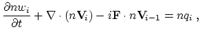
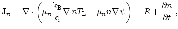
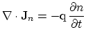
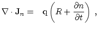
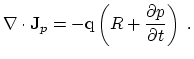
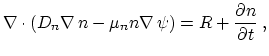
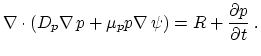
The analytical problem is basically formed by nonlinear partial differential equations. These equations are the Poisson equation (2.1) and the current continuity equations for the two carrier types in semiconducting materials, electrons and holes,
| (2.4) |
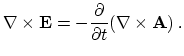
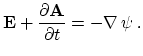
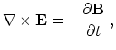
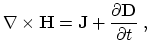
These three equations can be derived from the four Maxwell equations [100]:
![]() is related to the electric field
is related to the electric field
![]() by the permittivity tensor
by the permittivity tensor
![]() (assumed to be a scalar
(assumed to be a scalar
![]() hereafter):
hereafter):
 |
(2.10) |
 |
(2.11) |
| (2.12) |
The Poisson equation without considering a magnetic field is finally obtained by
| (2.14) |
The continuity equation for the conduction current density is derived by applying the divergence operator to (2.7) and using (2.8):
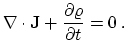 |
(2.15) |
Whereas the Maxwell equations can be used to derive the Poisson equation and the current continuity equations, the current relations cannot be derived from them. The carrier transport equations are therefore discussed in the next sections.
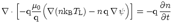
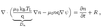
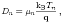
Many causes of the current flows can be identified, for example gradients of the carrier concentrations, temperatures or material properties or a contribution determined by Ohm's law [137,138]. The latter component is called drift current and can be formulated as
| (2.18) |
| (2.20) |
 |
(2.25) |
 |
(2.26) |
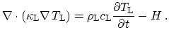
Nonlinear partial differential equations of second-order can appear in three variants: elliptic, parabolic, and hyperbolic. The Poisson equation as well as the steady-state continuity equations form a system of elliptic partial differential equations, whereas the lattice heat-flow equation is parabolic.
This can be shown for the Poisson equation posed in a bounded
domain
![]() by rewriting the differential operators of
(2.21) in (2.27) and for Cartesian coordinates
in (2.28), which is then compared with a general partial
differential equation of second order
(2.29):
by rewriting the differential operators of
(2.21) in (2.27) and for Cartesian coordinates
in (2.28), which is then compared with a general partial
differential equation of second order
(2.29):
| (2.30) |
To completely determine the solution of an elliptic partial differential equation boundary conditions have to be specified. Since parabolic and hyperbolic partial differential equations describe evolutionary processes, time normally is an independent variable and an initial condition is additionally required. As the transient continuity equations are parabolic, they require such an initial condition.
Macroscopic transport models can be systematically derived from the Boltzmann transport equation [134]
The distribution function ![]() as solution of (2.31) is used to obtain
the probability of finding a carrier inside a phase-space volume
as solution of (2.31) is used to obtain
the probability of finding a carrier inside a phase-space volume
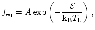
![]() . The equilibrium distribution function is the
Fermi-Dirac distribution. If the Pauli
exclusive principle is neglected, the
Maxwell distribution is obtained. In the drift-diffusion model the
cold and in the energy-transport the heated Maxwell distribution is
used. The six moments model uses an analytical distribution function in the
approach pursued here [84].
. The equilibrium distribution function is the
Fermi-Dirac distribution. If the Pauli
exclusive principle is neglected, the
Maxwell distribution is obtained. In the drift-diffusion model the
cold and in the energy-transport the heated Maxwell distribution is
used. The six moments model uses an analytical distribution function in the
approach pursued here [84].
This can be performed either directly by Monte Carlo simulations [112,115,123,122] or by the methods based on the expansion of the distribution function in momentum space into a series of spherical harmonics [97].
Monte Carlo simulations are particularly useful to obtain a physically accurate picture including various effects with as few approximations as possible. Since the simulations require much computational resources in terms of time and memory, it is rarely used on an engineering level. The extraction of small-signal parameters is often prohibitively costly, because the evaluation of a small-signal perturbation requires a low variance in the results.
Whereas for extremely small devices with gate lengths below 10![]() nm systems
based on the Wigner-Boltzmann equation
[151,149,150,70] have been applied, the ballistic limit
has been investigated by using transport models based on the
Schrödinger [124] equation.
nm systems
based on the Wigner-Boltzmann equation
[151,149,150,70] have been applied, the ballistic limit
has been investigated by using transport models based on the
Schrödinger [124] equation.
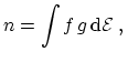
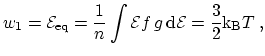
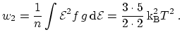
As its direct solution requires considerable computational resources, simpler
solutions are obtained by investigating lower moments of the distribution
function only. These include the electron concentration ![]() , the electron
temperature
, the electron
temperature
![]() , and the electron kurtosis
, and the electron kurtosis
![]() .
.
By multiplying (2.31) with a weight function
![]() and integrating
the result over the
and integrating
the result over the
![]() space, the macroscopic transport equations are
obtained. It is assumed that the Brillouin zone extends towards
infinity, which is justified due to the exponential decline of the distribution
function [240]. This procedure results in the following partial
differential equations in (
space, the macroscopic transport equations are
obtained. It is assumed that the Brillouin zone extends towards
infinity, which is justified due to the exponential decline of the distribution
function [240]. This procedure results in the following partial
differential equations in (
![]() )
)
![$\displaystyle \displaystyle \frac{\displaystyle \partial n \ensuremath{\langle ...
...emath{\mathbf{k}})] \,\, \mathrm{d}^3 \ensuremath{\mathbf{k}}} \ ,%\bestkiiint
$](img221.png) |
(2.32) |
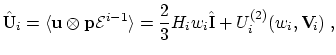
For the balance and flux equations, the weight functions
![]() and
and
![]() with the momentum
with the momentum
![]() are often used
[84]. For the drift-diffusion transport model, the
expansion is truncated at
are often used
[84]. For the drift-diffusion transport model, the
expansion is truncated at ![]() , for the energy-transport transport model at
, for the energy-transport transport model at ![]() ,
and eventually for the six moments transport model at
,
and eventually for the six moments transport model at ![]() . The balance and flux
relations read as follows [83]:
. The balance and flux
relations read as follows [83]:
| (2.39) |
![$\displaystyle n q_i = \ensuremath{\int {\mathcal{E}}^i \, Q[f(\ensuremath{\mathbf{k}})] \,\, \mathrm{d}^3 \ensuremath{\mathbf{k}}} \ ,$](img267.png) |
(2.40) |
![$\displaystyle n \ensuremath{\mathbf{Q}}_i = \ensuremath{\int \ensuremath{\mathb...
...\, Q[f(\ensuremath{\mathbf{k}})] \,\, \mathrm{d}^3 \ensuremath{\mathbf{k}}} \ .$](img268.png) |
(2.41) |
| (2.42) |
The moment ![]() is the carrier concentration,
is the carrier concentration,
![]() the average carrier
flux,
the average carrier
flux, ![]() the average energy,
the average energy,
![]() the average energy flux,
the average energy flux, ![]() the
average energy squared, and
the
average energy squared, and
![]() the average kurtosis flux.
the average kurtosis flux.
![]() is
the average carrier velocity,
is
the average carrier velocity,
![]() is the average momentum,
is the average momentum,
![]() the
energy tensor,
the
energy tensor,
![]() the second energy tensor, and
the second energy tensor, and
![]() is eventually the
third energy tensor. Furthermore it can be noted that (2.33) -
(2.38) are the continuity equation and current relation, the
energy balance and energy-flux relation, and the kurtosis balance and
kurtosis-flux relation, respectively.
is eventually the
third energy tensor. Furthermore it can be noted that (2.33) -
(2.38) are the continuity equation and current relation, the
energy balance and energy-flux relation, and the kurtosis balance and
kurtosis-flux relation, respectively.
As this equation system contains more unknowns than equations and each equation
is coupled to the next higher one, the so-called closure problem comes into
play: additional relations have to be introduced in order to close the equation
system, thus making it solvable. There are several approaches to overcome this
problem [84], for example the maximum entropy method
[129], Grad's method [80], the
cumulant closure method [176,235,192], or
a Maxwell closure [85]. The choice of
variables which are expressed by other ones is critical. The current density is
proportional to the average velocity
![]() . Furthermore, the average energy
. Furthermore, the average energy
![]() is used to model many physical effects. For that reason,
is used to model many physical effects. For that reason,
![]() and
and
![]() are chosen to remain as solution variables and the additional moments are
expressed as functions of the solution variables. According to
[82], the energy-like tensor
are chosen to remain as solution variables and the additional moments are
expressed as functions of the solution variables. According to
[82], the energy-like tensor
![]() are
are
 |
(2.43) |
 |
(2.46) |
 |
(2.47) |
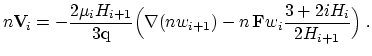
The fluxes can be explicitly written as
The non-parabolicity correction factors ![]() equal unity in the case of
parabolic bands and are modeled as either energy-dependent using a simple
analytical expression [28], by the incorporation of bulk Monte Carlo data
[84,219] or via analytic models for the distribution
function
[82].
equal unity in the case of
parabolic bands and are modeled as either energy-dependent using a simple
analytical expression [28], by the incorporation of bulk Monte Carlo data
[84,219] or via analytic models for the distribution
function
[82].
Note that (2.45) still contains the tensors
![]() which have to be
approximated by the unknowns of the equation system
which have to be
approximated by the unknowns of the equation system ![]() and
and
![]() . Finally, the following variable transformation according to
[86] is introduced:
. Finally, the following variable transformation according to
[86] is introduced:
 Maxwell Maxwell Maxwell Maxwell |
(2.49) |
 and and |
(2.53) |
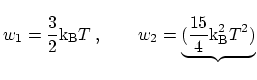
The equilibrium carrier temperature defined by (2.49) is different from the
lattice temperature, because a non-parabolic band structure is used. One
obtains
![]() and
and
![]() [84]. These are also the
values used for the Dirichlet boundary conditions for
[84]. These are also the
values used for the Dirichlet boundary conditions for ![]() and
and
![]() . For the carrier concentration a standard Ohmic contact
model is used, corresponding to a cold Maxwell distribution at the
contacts.
. For the carrier concentration a standard Ohmic contact
model is used, corresponding to a cold Maxwell distribution at the
contacts.
In the following sections, the transport models for the parabolic case are
used. Thus,
![]() ,
,
![]() , and
, and
![]() , resulting in
, resulting in
 |
(2.57) |
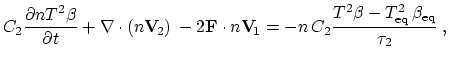
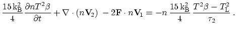
The closure of the six moments transport model at ![]() was determined as
was determined as
![]() . Thus, the following flux equations can be derived:
. Thus, the following flux equations can be derived:
 |
(2.64) |
 |
(2.65) |
 |
(2.66) |
 |
(2.67) |
By using the closure ![]() at
at ![]() , the flux equations of the energy-transport
transport model can be obtained:
, the flux equations of the energy-transport
transport model can be obtained:
| (2.68) | |
| (2.69) |
The balance equations are (2.61) and (2.62).
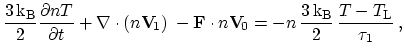
For the drift-diffusion transport model, the closure at ![]() was found to be
was found to be
![]() , yielding the following balance and flux equation:
, yielding the following balance and flux equation:
These equations look very familiar, as they were the result of the derivation
in Section 2.1.1. In the flux equation (2.70), the external force
is substituted by
![]() .
.
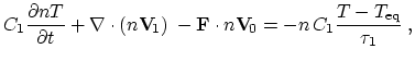
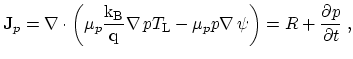
Eventually, (2.70) must be inserted into (2.71), which is the balance equation corresponding to (2.2).
 |
(2.72) |
 |
(2.73) |
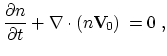
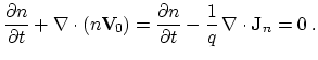
When
![]() is assumed to be constant, the isothermal drift-diffusion model as
already shown in (2.22) can be finally obtained:
is assumed to be constant, the isothermal drift-diffusion model as
already shown in (2.22) can be finally obtained:
 |
(2.74) |
 |
(2.75) |
![$\displaystyle \displaystyle \frac{\displaystyle \partial f}{\displaystyle \part...
..._{\negmedspace \ensuremath{\mathbf{p}}}} f} = Q[f(\ensuremath{\mathbf{k}})] \ .$](img209.png)