Subsections

• 2.3.1 Solving the Nonlinear System
• 2.3.2 Transient Simulation

2.3 Steady-State and Transient Analysis

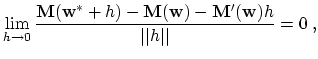
This section gives an overview about the steady-state and transient simulation modes including a discussion of the nonlinear solution technique. For the steady-state analysis, the discretized equations (2.21), (2.22), and (2.23) can be symbolically written as:

$${ F_{\psi}(\ensuremath{\ensuremath{\mathbf{w}}}) = 0\ ,$$ (2.99)

$$F_{n}(\ensuremath{\ensuremath{\mathbf{w}}}) = 0\ ,$$ (2.100)

$$F_{p}(\ensuremath{\ensuremath{\mathbf{w}}}) = 0\ ,{$$ (2.101)

with

$$\ensuremath{\mathbf{\ensuremath{\ensuremath{\mathbf{w}}}}} = \left( \begin{array}{c} \psi \\ n \\ p \end{array}\right) \ .$$ (2.102)

Note that for the sake of simplification, the vectors of the discretized quantities and equations are not explicitly noted. The resulting discretized problem is then usually solved by a damped Newton method which requires the solution of a linear equation system at each step. The result of the steady-state simulation mode is the operating point, which is a prerequisite for any subsequent transient or small-signal simulation.

2.3.1 Solving the Nonlinear System

As the resulting discretized equation system is still nonlinear, the solution $\ensuremath{\ensuremath{\mathbf{w}}}^*$, which is assumed to exist is obtained by applying a linearization technique. The nonlinear problem can be defined as

$$\ensuremath{\mathbf{F}}(\ensuremath{\ensuremath{\mathbf{w}}}) = \ensuremath{\mathbf{0}}\ ,$$ (2.103)

with

$$\ensuremath{\mathbf{F}}(\ensuremath{\ensuremath{\mathbf{w}}}) = \... ...athbf{w}}}) \\ F_p(\ensuremath{\ensuremath{\mathbf{w}}}) \end{array} \right)\ .$$ (2.104)

Most iterative methods are based on a fixpoint equation $\ensuremath{\ensuremath{\mathbf{w}}}= \ensuremath{\ensuremath{\mathbf{M}}(\ensuremath{\ensuremath{\mathbf{w}}})}$, where $\ensuremath{\ensuremath{\mathbf{M}}(\ensuremath{\ensuremath{\mathbf{w}}})}$ is constructed in such a way that the fixpoint $\ensuremath{\ensuremath{\mathbf{w}}}^*$ is a solution of that equation [193]. During the iteration the error between the current solution $\ensuremath{\ensuremath{\mathbf{w}}}^k$ of the $k$-th iteration step and $\ensuremath{\ensuremath{\mathbf{w}}}^*$ converges to zero, if specific properties and requirements on the initial guess $\ensuremath{\ensuremath{\mathbf{w}}}^0$ are fulfilled. With a neighborhood $S(\ensuremath{\ensuremath{\mathbf{w}}}^*)$, $\ensuremath{\ensuremath{\mathbf{M}}(\ensuremath{\ensuremath{\mathbf{w}}})} \in S$, $\ensuremath{\ensuremath{\mathbf{w}}} \in S$ and a constant $\alpha \in [0,1[$, the iteration will converge for any $\ensuremath{\ensuremath{\mathbf{w}}}^0 \in S(\ensuremath{\ensuremath{\mathbf{w}}}^*)$ to $\ensuremath{\ensuremath{\mathbf{w}}}^*$, if

$$\vert\vert\ensuremath{\ensuremath{\mathbf{M}}(\ensuremath{\ensure... ...{w}}}^* \vert\vert \ , \forall \, \ensuremath{\ensuremath{\mathbf{w}}}\in S \ .$$ (2.105)

Then, $\ensuremath{\ensuremath{\mathbf{M}}(\ensuremath{\ensuremath{\mathbf{w}}})}$ is a so-called contractive mapping, and the locally convergent iteration does converge for any $\ensuremath{\ensuremath{\mathbf{w}}}^0 \in S$ to $\ensuremath{\ensuremath{\mathbf{w}}}^*$. In order to fulfill (2.105) it is assumed that the Frechet derivative $\ensuremath{\ensuremath{\mathbf{M}}'(\ensuremath{\ensuremath{\mathbf{w}}})}$ exists at the fixpoint $\ensuremath{\ensuremath{\mathbf{w}}}^*$ and that its eigenvalues are less than one in modulus [193]. According to the Ostrowski theorem [243], $\ensuremath{\ensuremath{\mathbf{M}}(\ensuremath{\ensuremath{\mathbf{w}}})}$ is contractive if the spectral radius $\rho(\ensuremath{\ensuremath{\mathbf{M}}'(\ensuremath{\ensuremath{\mathbf{w}}})}) < 1$, which is the maximal modulus of all eigenvalues of $\ensuremath{\ensuremath{\mathbf{M}}(\ensuremath{\ensuremath{\mathbf{w}}})}$. If $\ensuremath{\ensuremath{\mathbf{M}}'(\ensuremath{\ensuremath{\mathbf{w}}})}$ exists such that

$$\lim_{h \rightarrow 0} \frac{\ensuremath{\ensuremath{\mathbf{M}}(... ...{M}}'(\ensuremath{\ensuremath{\mathbf{w}}})} h}{\vert\vert h\vert\vert} = 0 \ ,$$ (2.106)

$\ensuremath{\mathbf{M}}'(\ensuremath{\ensuremath{\mathbf{w}}})$ is the Frechet derivative. The most prominent of such linearization techniques is the Newton method [136] based on a Taylor series expansion. It can be written in the form [193,201]:

$$- \ensuremath{\mathbf{J}}(\ensuremath{\ensuremath{\mathbf{w}}}) \... ...rray}\right) = \ensuremath{\mathbf{f}}(\ensuremath{\ensuremath{\mathbf{w}}})\ ,$$ (2.107)

where $\ensuremath{\mathbf{J}}(\ensuremath{\ensuremath{\mathbf{w}}})$ is the Jacobian matrix with the first partial derivatives [136]:

$$\ensuremath{\mathbf{J}}(\ensuremath{\ensuremath{\mathbf{w}}}) = \... ...\frac{\displaystyle \partial F_p}{\displaystyle \partial p} \end{array} \right)$$ (2.108)

As the iteration can be rewritten in the form

$$\ensuremath{\ensuremath{\mathbf{w}}}^{k+1} = \ensuremath{\ensurem... ...bf{J}}^{-1} \ensuremath{\mathbf{F}}(\ensuremath{\ensuremath{\mathbf{w}}}^k) \ ,$$ (2.109)

the Frechet derivative evaluated at $\ensuremath{\ensuremath{\mathbf{w}}}^*$ equals $\ensuremath{\mathbf{I}} - \ensuremath{\mathbf{J}}(\ensuremath{\ensuremath{\mathbf{w}}}^*) \ensuremath{\mathbf{F}}'(\ensuremath{\ensuremath{\mathbf{w}}}^*)$ resulting in $\rho = 0$. Hence, the Newton method converges for all $\ensuremath{\ensuremath{\mathbf{w}}}^0$ sufficiently close to $\ensuremath{\ensuremath{\mathbf{w}}}^*$.

It is important to note that $\ensuremath{\mathbf{J}}$ must only be an approximation of the Frechet derivative, which follows from the derivation of $\rho$ [193]. Furthermore, in order to enlarge the radius of convergence and thus improve the convergence behavior of the Newton approximation, the couplings between the equations can be reduced, especially during the first steps of the iteration. Before the update norm, that is the infinity norm of the update vectors of all quantities, has fallen below a specified value, the derivatives as shown in Table 2.1 are normally ignored. Besides the driving force for electrons and holes in the drift-diffusion model, $F_n$ and $F_p$, and the tunneling current density $J_\mathrm{tun}$, all quantities are already known from the previous sections. Note that for the sake of simplification just the symbols are given without vector notations.

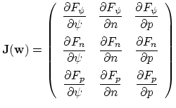
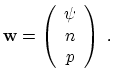
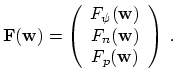
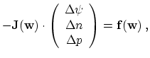
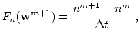
Table 2.1: Ignored derivatives during the first steps of the Newton iteration.

	$$\psi$$	$n$	$p$	$$\ensuremath{T_n}$$	$$\ensuremath{T_p}$$	$$\ensuremath{\beta_n}$$	$$\ensuremath{\beta_p}$$	$$F_n$$	$$F_p$$
$J_n$				$$\displaystyle \frac{\displaystyle \partial J_n}{\displaystyle \partial \ensuremath{T_n}}$$				$$\displaystyle \frac{\displaystyle \partial J_n}{\displaystyle \partial F_n}$$
$J_p$					$$\displaystyle \frac{\displaystyle \partial J_p}{\displaystyle \partial \ensuremath{T_p}}$$				$$\displaystyle \frac{\displaystyle \partial J_p}{\displaystyle \partial F_p}$$
$S_n$	$$\displaystyle \frac{\displaystyle \partial S_n}{\displaystyle \partial \psi}$$			$$\displaystyle \frac{\displaystyle \partial S_n}{\displaystyle \partial \ensuremath{T_n}}$$		$$\displaystyle \frac{\displaystyle \partial S_n}{\displaystyle \partial \ensuremath{\beta_n}}$$
$S_p$	$$\displaystyle \frac{\displaystyle \partial S_p}{\displaystyle \partial \psi}$$				$$\displaystyle \frac{\displaystyle \partial S_p}{\displaystyle \partial \ensuremath{T_p}}$$		$$\displaystyle \frac{\displaystyle \partial S_p}{\displaystyle \partial \ensuremath{\beta_p}}$$
$R$	$$\displaystyle \frac{\displaystyle \partial R}{\displaystyle \partial \psi}$$	$$\displaystyle \frac{\displaystyle \partial R}{\displaystyle \partial n}$$	$$\displaystyle \frac{\displaystyle \partial R}{\displaystyle \partial p}$$
$\mu_n$								$$\displaystyle \frac{\displaystyle \partial \mu_n}{\displaystyle \partial F_n}$$
$\mu_p$									$$\displaystyle \frac{\displaystyle \partial \mu_p}{\displaystyle \partial F_p}$$
$J_\mathrm{tun}$	$$\displaystyle \frac{\displaystyle \partial J_\mathrm{tun}}{\displaystyle \partial \psi}$$	$$\displaystyle \frac{\displaystyle \partial J_\mathrm{tun}}{\displaystyle \partial n}$$	$$\displaystyle \frac{\displaystyle \partial J_\mathrm{tun}}{\displaystyle \partial p}$$	$$\displaystyle \frac{\displaystyle \partial J_\mathrm{tun}}{\displaystyle \partial \ensuremath{T_n}}$$	$$\displaystyle \frac{\displaystyle \partial J_\mathrm{tun}}{\displaystyle \partial \ensuremath{T_p}}$$

The linear equation system for the $k$-th iteration step looks like:

$$- \ensuremath{\mathbf{J}}^k \ensuremath{\mathbf{x}}^{k+1} = \ensuremath{\mathbf{F}}(\ensuremath{\ensuremath{\mathbf{w}}}^k)\ .$$ (2.110)

The right-hand-side vector $\ensuremath{\mathbf{F}}(\ensuremath{\ensuremath{\mathbf{w}}}^k)$ is the residual and $\ensuremath{\mathbf{x}}^{k+1}$ is the update and correction vector. This solution vector $\ensuremath{\mathbf{x}}$ of the linear equation system is used to calculate the next solution $\mathbf{w}$ of the Newton approximation:

$$\ensuremath{\mathbf{w}}^{k+1} = \ensuremath{\mathbf{w}}^k + \ensuremath{\mathbf{x}}^{k+1}\ .$$ (2.111)

To avoid overshoot of the solution and to extend the local convergence of the method several damping schemes suggested by Deuflhard [50] or Bank and Rose [15] can be used to calculate a damping factor $D$. The damped update reads

$$\ensuremath{\mathbf{w}}^{k+1} = \ensuremath{\mathbf{w}}^k + D \, \ensuremath{\mathbf{x}}^{k+1}\ .$$ (2.112)

Investigations have shown that damping based on the potential delivers the most promising results [65]:

$$D = \displaystyle \frac{1+\delta\cdot\ln\frac{\displaystyle \Vert... ...style V_\mathrm{th}}-1\right)} \ , \qquad \mathrm{with} \quad 0 \leq \delta \ ,$$ (2.113)

where $\delta$ is an adjustable parameter of the damping scheme, $\ensuremath{\mathbf{x}}_\psi$ the update norm of the potential sub-vector, and $V_\mathrm{th}$ the thermal voltage. Larger $\delta$ yields more logarithm-like damping. The potential damping scheme avoids the expensive evaluation of the right-hand-side vector, which is for example required for the scheme of Bank and Rose [15].

2.3.2 Transient Simulation

The transient problem arises if the boundary condition for the electrostatic potential or the contact currents becomes time-dependent. Hence, the partial time derivatives of the carrier concentrations in (2.22) and (2.23) have to be taken into account.

There are several approaches for transient analysis [193], among them are the forward and backward Euler approaches. Whereas the former shows significant stability problems, the latter is unconditionally stable for arbitrarily large time steps $\Delta t$. However, full backward time differencing requires much computational resources for solving the large nonlinear equation system at each time step, but gives good results. The quality of the results can be measured by the truncation error [146]. Equations (2.21), (2.22) and (2.23), discretized in time and symbolically written, read then at the $m$-th time step when $m+1$ is to be calculated:

$${ F_{\psi}(\ensuremath{\ensuremath{\mathbf{w}}}^{m+1}) = 0\ ,$$ (2.114)

$$F_{n}(\ensuremath{\ensuremath{\mathbf{w}}}^{m+1}) = \frac{n^{m+1} - n^m}{\Delta t}\ ,$$ (2.115)

$$F_{p}(\ensuremath{\ensuremath{\mathbf{w}}}^{m+1}) = \frac{p^{m+1} - p^m}{\Delta t}\ . {$$ (2.116)

From a computational point of view it is to note, that in comparison to the steady-state solution the algebraic equations arising from the time discretization are significantly easier to solve [193]. This has mainly two reasons: first, the partial time derivatives help to stabilize the spatial discretization. Second, the solutions can be used as a good initial guess for the next time step. Furthermore, the equation assembly structures can be reused (see Section 4.12).