3.6 Combination of Monte Carlo Method with Direct Calculation

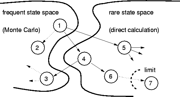
    Consider all possible states as divided into two subspaces, the  frequent state space and the  rare state space, as shown in Fig. 3.9.

  

Figure 3.9: Partition of the state space into a frequent and a rare state domain.

The MC part simulates only the frequent state space, which gives the occupation probabilities of frequent states. The occupation probability P_i is calculated as the ratio of time T_i spent in state i to the total simulation time $T_{\Sigma}$.
$$\begin{gather}P_i = \frac{T_i}{T_{\Sigma}} \qquad\text{with}\qquad T_{\Sigma} = \sum_i T_i \end{gather}$$
P_i is the solution to the stationary ME for the frequent states. Instead of waiting for the MC simulator to step into the rare state space, which would result in impractically long simulation times, we directly calculate the contribution of events leading to rare states by stepping through the  event tree (see Fig. 3.10) starting at frequent states.

  

Figure 3.10: Direct calculation of the contribution of rare states and events by stepping through the event tree. Solid arrows mark transitions that are considered for the direct calculation part.

The essential assumption is that the rare states cause only a small perturbation to the frequent state probabilities.
$$\begin{gather}\sum_j T_{j,rare} \ll T_{\Sigma}, \end{gather}$$
where T_j,rare is the time spent in the rare state j, which can be directly calculated from the stationary ME.
$$\begin{gather}T_{j,rare} = \frac{\sum_{i\neq j} (T_i \Gamma_{ji})}{\sum_{k\neq j} (\Gamma_{kj})} \end{gather}$$
$T_i \Gamma_{ji}$ is the number of times the rare state j would be in average visited from state i, $\sum_{k\neq j}\Gamma_{kj}$ is the exit rate of state j and thus $1/\sum_{k\neq j}\Gamma_{kj}$ is the average time spent in state j for one visit. We are using time averages for the direct calculation. Actually the durations are distributed with a Poisson distribution. However, the directly calculated rare state space is only a small perturbation to the frequent state space which is calculated with a MC method where the Poisson distribution of the tunnel durations is fully incorporated. The occupation probability for a rare state is therefore
$$\begin{gather}P_{j,rare} = \frac{T_{j,rare}}{T_{\Sigma}} = \frac{\sum_{i\neq j} (T_i \Gamma_{ji})}{\sum_{k\neq j} (\Gamma_{kj}) \;T_{\Sigma}}. \end{gather}$$
The algorithm follows all possible events starting at frequent states. If a frequent state is encountered the algorithm terminates that branch, because the state probability is already known. Once the probability of a state is lower than a predefined limit no further descent into following branches from this state is made (see Fig. 3.10).