The Basic Semiconductor Equations

4.1 The Basic Semiconductor Equations

The basic semiconductor equations [1] consist of the Poisson equation (Equation 4.1),

∇ ⋅(ε⋅∇ φ) = q(n− p− N + N ) D A

(4.1)

the continuity equations for electrons (Equation 4.2) and holes (Equation 4.3),

∂n- ∇ ⋅Jn − q ∂t = qR

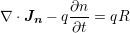(4.2)

∂p- ∇ ⋅Jp + q ∂t = − qR

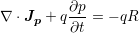(4.3)

as well as the current relations for electrons (Equation 4.4) and holes (Equation 4.5)

Jn = − qμn (n∇ φ− VT∇n )

(4.4)

J = − qμ (p∇φ + V ∇p ) p p T

(4.5)

based on the DD model [103].

$ε$ denotes the permittivity, $q$ the elementary charge, $ND$ the donor doping concentration, and $NA$ the acceptor doping concentration. With respect to the continuity equations and the current relations, $Jn$ refers to the electron current density, $Jp$ the hole current density, $R$ the recombination rate, and $VT$ the thermal voltage.

The DD model considers two charge transport mechanisms, those being charge carrier drift and diffusion, respectively. In general, charge carrier drift due to the presence of an electric field, implemented by the first term of the DD model, containing the gradient of the potential. On the contrary, diffusion is a fundamental process, which aims to establish a thermodynamic equilibrium in an initially imbalanced physical system. In the case of semiconductor physics, diffusion is achieved by carrier migration from areas with high concentration to areas where the concentration of particles is lower. Therefore, the DD model includes the second term, incorporating the gradient of the charge carrier concentration.

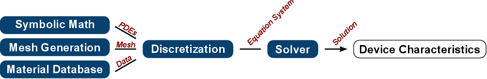
Substituting the current densities in the continuity equations (Equations 4.2-4.3) for the current relations (Equations 4.4-4.5) yields a system of three partial differential equations ( PDEs), coupled via the potential $φ$ , the electron concentration $n$ , and the hole concentration $p$ . These PDEs are typically discretized with the finite volume method to conserve the current [1], stabilized by the Scharfetter-Gummel discretization [104], and solved via nonlinear iterative solvers, such as the Newton scheme or the Gummel method [1]. The solved potential, electron concentration, and hole concentration distributions are used to compute, for instance, the current densities, essential to evaluating the device performance via the current-voltage characteristics, where the evaluated current at terminal contacts is related to the individually applied terminal voltages.

Although the basic semiconductor equations were successfully applied in the last decades, with the continuing shrinking of the device dimensions the typically applied DD model struggles to provide reasonable predictions [46]. Therefore, additional models have been developed [105], underlining the need for a modern device simulation software to support an exchangeable and expandable modeling backend.

As the focus of this work is on investigating approaches for a flexible device simulation framework, the actual transport model required for conducting device simulations is of marginal importance. Therefore, the simple yet representative DD transport model is sufficient for the subsequent investigations.

pict

Figure 4.2: The essential components of a device simulator are shown. The discretization scheme assembles an equation system according to the defined PDEs, the input mesh, and the required material data. The equation system is solved via a solver component, computing the solution from which the device characteristics is derived.

[next] [prev] [prev-tail] [front] [up]