In common, anisotropy is understood as the condition of holding a property
value being dependent on the directions in which it is observed. For better
understanding of the term anisotropy in the context of
tetrahedral meshes first a definition for mesh density is given. Second,
a novel approach is presented of how anisotropy can be seen as property of a
single tetrahedron and how this property can be visualized.
Afterwards an extension of the recursive tetrahedral bisection algorithm,
presented in Section 2.2.3, is depicted, which can largely benefit from
the incorporation of an anisotropic metric.
In general anisotropy in context of tetrahedral meshes can be seen as
direction-dependent variation of mesh density (see
Definition 12).
Mapping this idea on a tetrahedron, anisotropy can be understood
as variation of the coordinate system related distances between the
vertices. This thought is based on a method which is a well-known statistical
technique called Principal Component Analysis (PCA) [46].
PCA is a useful method that has found
application in many scientific areas, such as, image
analysis and compression, face recognition, and regression. PCA is also a
common technique for finding patterns in data of high
dimensions [47].
Appendix A gives a full representation on how PCA is used to find a quantitative description for the geometric property of a tetrahedron. However, PCA analysis for a tetrahedron forms a quadratic surface which can be used as measure for anisotropy, i.e. roughly speaking if PCA comes up with a sphere the tetrahedra is more regular (isotropy). If it forms an ellipsoid, than the tetrahedron is said to be anisotropic, see Figure 2.5.
![\begin{figure*}\setcounter{subfigure}{0}
\centering
\subfigure[Anisotropy.]
{\...
...epsfig{figure=pics/PCA-Regular.eps2,height=0.25\textwidth}}% \\
\end{figure*}](img129.png) |
In the following it is shown, how regular, mostly isotropic meshes can be
transformed by refinement into anisotropic meshes.
The idea is based on the introduction of a tensor-based metric space, representing
mesh anisotropy over the domain [48], which controls a modified tetrahedral
bisection algorithm.
Based on the ideas discussed in Section 2.3 we want to go the other way around and start with a definition of the term metric and how a tensor function can be used to form a non-constant anisotropic metric space.
For a better understanding of the following I also want to give a definition for a metric tensor [51].
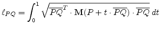
Applying this metric to tetrahedral meshes means that
calculating the edge length of an element in a metric space can be seen
as calculating a line integral.
An arc length ![]() is defined as the length along
a curve
is defined as the length along
a curve ![]() :
:
![]() .
The length of a line
segment
.
The length of a line
segment
![]() in a metric space is calculated by
in a metric space is calculated by
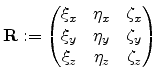
The idea now is to apply a combination of coordinate system rotation
![]() (see Appendix B.1) and dilation defining the
anisotropic metric function
(see Appendix B.1) and dilation defining the
anisotropic metric function
![]() , where
the dilation is represented by three scalar values
, where
the dilation is represented by three scalar values
![]() and
and
![]() , respectively.
, respectively.
Using
![]() as an orthogonal coordinate system
and the dilation values
as an orthogonal coordinate system
and the dilation values
![]() we define two matrices
we define two matrices
In general a tensor
![]() formed by a
formed by a
![]() matrix can
be split into a symmetric
matrix can
be split into a symmetric
![]() and an antisymmetric part
and an antisymmetric part
![]() such that
such that
![]() where
where
![]() and
and
![]() [52]. The antisymmetric part in essence
describes a rotation merely, so the following deals with symmetric, second
order tensors only.
[52]. The antisymmetric part in essence
describes a rotation merely, so the following deals with symmetric, second
order tensors only.
According to matrix
![]() and matrix
and matrix
![]() the metric tensor can be seen
as three-dimensional distortion of a sphere. For example, in a simple case, where
the rotation matrix
the metric tensor can be seen
as three-dimensional distortion of a sphere. For example, in a simple case, where
the rotation matrix
![]() is equal to the identity matrix
is equal to the identity matrix
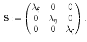
![]() and the distortion matrix is set as
and the distortion matrix is set as
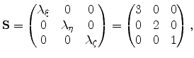 |
(2.9) |
an initial sphere is transformed to an ellipsoid, which represents
the new metric (compared to the undistorted Euclidean metric) measurement units
of the distorted space.
This point of view is depicted in
Figure 2.6 and Figure 2.7, respectively.
For the visualization of pointwise defined second order
tensor functions a so-called glyph-based, more exactly, a metric
ellipsoids glyph-based approach [53] is used which is described in
detail in Appendix A.3.
In Figure 2.7 one can see,
that there is no distortion along the ![]() -axis. In the
-axis. In the ![]() -direction the space is
stretched by a factor of three and in
-direction the space is
stretched by a factor of three and in ![]() -direction by a factor of
two. According to formula (2.2) the square length of an edge
-direction by a factor of
two. According to formula (2.2) the square length of an edge
![]() which is oriented exactly
which is oriented exactly ![]() -directional appears three times
longer then the same edge measured in an undistorted Euclidian space (where the
metric tensor function
-directional appears three times
longer then the same edge measured in an undistorted Euclidian space (where the
metric tensor function
![]() is equal to the identity matrix
is equal to the identity matrix
![]() ).
).
In this simplified case the rotation matrix was set to the
identity matrix
![]() and therefore, the distorted space and the undistorted
space are collateral. Please notice that the metric tensor function in this
example does not vary over the space and is therefore constant:
and therefore, the distorted space and the undistorted
space are collateral. Please notice that the metric tensor function in this
example does not vary over the space and is therefore constant:
![]() .
.
![\includegraphics[width=0.75\textwidth]{pics/iso.eps2}](img177.png)
|
![\includegraphics[width=0.75\textwidth]{pics/aniso.eps2}](img179.png)
|
With the help of the anisotropy metric function defined in
Section 2.3.1 and the bisection algorithm presented in
Section 2.2.2, an anisotropic tetrahedral bisection algorithm can be
derived.
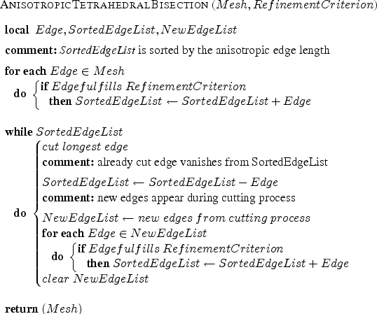
The basic idea behind this refinement procedure is to calculate the length of all edges marked for refinement in a given metric and to determine the longest anisotropic edge according to the metric function through formula (2.2). Afterwards, the longest anisotropic edge is cut into two pieces of equal (isotropic measured) length. During this cutting process all new edges must also be taken into consideration. Now the procedure starts again by marking edges according to the refinement criterion and stops if there is no edge which fulfills the criterion anymore. Table 2.2 gives a pseudo-code fragment which shows the nature of this algorithm.
The complexity of the algorithm depends mostly on the amount of edges
produced during the cutting process. This is in general unknown and can only be
calculated exactly subsequently. Under the assumptions that the initial mesh carries
![]() -edges,
-edges, ![]() -edges are marked for refinement, and
-edges are marked for refinement, and ![]() -edges are born during
the overall refinement process, the complexity has the bounded order of
-edges are born during
the overall refinement process, the complexity has the bounded order of
![]() .
.
One open item is the RefinementCriterion-function used in the
anisotropic tetrahedral bisection algorithm, depicted in Table 2.2.
One has to distinguish between pure geometric RefinementCriterion-functions and
so-called data driven RefinementCriterion-functions which are subject of
Section 3. Pure geometric RefinementCriterion-functions come to a decision only by
analyzing geometric properties of the refinement edge and all associated mesh
elements. The recursive tetrahedral bisection algorithm presented in
Section 2.2.3 is a member of this class.
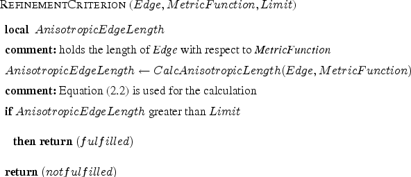
The simplest case for a RefinementCriterion-function under consideration of a given metric function
is shown in Table 2.3. In this particular case the length of the refinement
edge is calculated related to a given MetricFunction
![]() with
respect to Equation (2.2). As second step a maximum edge length limit
is introduced, which bounds the anisotropic length of each edge. If the length
exceeds the limit, the edge is marked for refinement otherwise not.
with
respect to Equation (2.2). As second step a maximum edge length limit
is introduced, which bounds the anisotropic length of each edge. If the length
exceeds the limit, the edge is marked for refinement otherwise not.
Strictly speaking this RefinementCriterion-function is already a data driven refinement method, because the metric function itself is analyzed for the refinement decision and so not only pure geometric properties are used. However, in Section 3 different data driven RefinementCriterion-functions are derived, which enables a powerful anisotropic mesh refinement technique for several simulation tasks for TCAD tools.
 and
and