Subsections

• 3.2.1 Laplace Equation
• 3.2.2 Plate Capacitor
• 3.2.3 Metric Function
• 3.2.4 Propaedeutic Example

3.2 Layer Refinement Method

Typical processing steps involved in the fabrication of semiconductor devices can be arranged into four groups [56], namely pattern definition like lithography, pattern transfer like etching, layer formation like oxidation or deposition, and layer modification like diffusion or ion implantation. Common to all these fabrication procedures is the fact, that each step itself hardly influences only a particular region, a geologist would say a particular stratum of the machining wafer. Other regions are only slightly or very often negligibly small effected. These actualities gives rise to the layer refinement method which is used to introduce a region of higher mesh density into an existing mostly coarse mesh.

The following deals with the design of a refinement method which has the ability of anisotropic refinement for well defined surface layers with an adjustable thickness. The basic idea is to use a metric tensor function (see Section 2.3.1) which is derived from data stored on the initial mesh to control an anisotropic tetrahedral bisection process (see Section 2.3.2).

To determine surface layers, one hast to calculate the Euclidian distance to each vertex in the interior of the mesh domain to the surface. This problem is well-known and can be found in literature as distance transform or distance map, which is normally only applied to binary images. The extension to three dimensions is not trivial, especially for unstructured tetrahedral meshes. A promising technique for solving this problem can found in [57], which deals with propagating surfaces. However, the drawback of this method is the need of a special representation of vertex polyhedra, which increases the memory demand dramatically.

Therefore in this work the solution of Laplace's equation as approximation for the surface distance map is chosen. This approach is, compared to the pure calculation of the distance transform, more flexible and can also handle multiple segment domains with appropriate interface conditions.

3.2.1 Laplace Equation

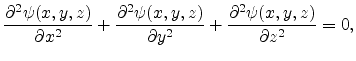
The three-dimensional Laplace equation in the Cartesian coordinate system is the second order partial differential equation given by

$$\frac{\partial^2\psi (x,y,z)}{\partial x^2}+\frac{\partial^2\psi (x,y,z)}{\partial y^2}+\frac{\partial^2\psi (x,y,z)}{\partial z^2} = 0,$$ (3.8)

which is often written as

$$\triangle \psi (x,y,z) = \nabla^{2}\psi (x,y,z) = \operatorname{div}\operatorname{grad} \psi (x,y,z) = 0,$$ (3.9)

where $\operatorname{div}$ is the divergence, $\operatorname{grad}$ is the gradient, and $\triangle$ is the Laplace operator.

A function $\psi (x,y,z)$ which satisfies the Laplace equation is said to be harmonic and analytic within the domain where the equation is satisfied. Solutions do not have any local maxima or minima. Because the Laplace equation is linear, the superposition of any two solutions is also a solution. A solution is determined uniquely, if appropriate boundary conditions are posed [58].

The problem of finding a solution $\psi (x,y,z)$ on some spatial domain $\mathcal{V}$ with respect to a given function defined on the boundary $\partial \mathcal{V}$ is called Dirichlet problem. Neumann boundary conditions imposed on partial differential equation specify a vanishing normal derivative [59]. Typically a mixture of Dirichlet and Neumann boundary conditions is used.

3.2.2 Plate Capacitor

As said, the idea is to use the solution of the Laplace equation as an approximation for a surface distance function. The imagination is based on electrostatic field calculations of the plate-capacitor [60] (see Figure 3.5). A typical plate-capacitor structure is formed by two coplanar metal planes that are connected to a voltage supply. We neglect the surrounding area by applying Neumann boundary conditions at the open borders of the capacitor and Dirichlet boundary conditions at the electrodes (assumes an infinitely expanded capacitor).

Figure 3.5: Figure 3.5(a) shows a typical plate-capacitor structure. Two coplanar metal planes are connected to a voltage supply. The lower plane is riddled with a bead. The resulting electrostatic field is shown in 3.5(b). The electrical field is a vector quantity which is perpendicular to the iso-surfaces of the electrostatic potential $\psi$ (picture adapted from [60]).

Iso-surfaces of the electrostatic potential inside the plate-capacitor also form coplanar planes which can be used as a measure for the perpendicular distance to the surface. This measure is exact, if and only if the plates are coplanar. For non-planar structures, the electrostatic potential is only an approximation for the surface distance (see Figure 3.5(b)). In technical terms, the electrical field $\vec{E}$ can be written as a gradient field of the electrostatic potential $\psi$ :

$$\vec{E}=-\vec{\nabla}\psi.$$ (3.10)

3.2.3 Metric Function

As shown in Section 2.3.1 and Section 2.3.2 a tensor function of second order $\mathbf{M}^{3 \times 3}(x,y,z)$ can be used to control an anisotropic tetrahedral bisection refinement process. Now the solution $\psi (x,y,z)$ of the Laplace equation as approximation for the surface distance field and an arbitrary element grading function $f(\psi )$ is used to construct such a metric tensor function $\mathbf{M}^{3 \times 3}=\mathbf{M}(x,y,z,f(\psi))$ . Based on this combination the so-called layer refinement method can be introduced, since the iso-levels of the Laplace equation solution define ``laminated regions''.

To depict this process in action a propaedeutic example is used later on, where starting from a coarse mesh of an eighth of a sphere a finer mesh layer near the spike at the center is introduced (see Figure 3.7 for the initial mesh).

Based on the two matrices $\mathbf{R}$ and $\mathbf{S}$ the metric function is defined by $\mathbf{M}=\mathbf{R}\mathbf{S}\mathbf{R}^T$ , as depicted in Section 2.3.1, Equation (2.3). For the layer refinement method the rotation matrix $\mathbf{R}$ is set to the identity matrix $\mathbf{I}$ . This causes an equal weighting in all directions and therefore a special case of anisotropic refinement, namely the isotropic refinement. This means that the refinement procedure is directionally independent, the only dependence is given by the grading function $f(\psi )$ .

For the dilation factor, represented by the matrix $\mathbf{S}$ , the following interrelationship is applied:

$$\mathbf{S} =\begin{pmatrix}\lambda_{\xi} & 0 & 0 \ 0 & \lambda_{... ...in{pmatrix}f(\psi) & 0 & 0 \ 0 & f(\psi) & 0 \ 0 & 0 & f(\psi) \end{pmatrix}.$$ (3.11)

Back to the imagination of the plate-capacitor for the surface layer refinement, we want to define a region of finer mesh near higher potential values, because these potential values are ``closer''to the surface, since the solution of the Laplace equation has the only minima and maxima at the boundary of the domain. Other regions should be not effected by the refinement procedure, so the dilation function should deliver almost no dilation in domains with lower ``potential''.

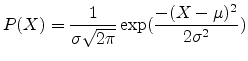
For the construction of such a dilation function $\lambda = f(\psi)$ experiments have shown that functions with the shape of a Gaussian probability distribution (also known as Gaussian ``bell curve''), see Remark 3, are good choices for a smooth and well adjustable dilation function $f(\psi )$ but other functions are conceivable.

Remark 3 (Gaussian Probability Distribution)   A normal distribution in a variate $X$ with mean $\mu$ and variance $\sigma{}^{2}$ is a statistic distribution with probability function

$$P(X)=\frac{1}{\sigma \sqrt{2 \pi}}\exp({\frac{-(X-\mu)^{2}}{2 \sigma{}^2}})$$ (3.12)

on the domain $X \in (-\infty{},\infty{})$ .

Figure 3.6: Dilation function $f(\psi )$ for stretching parameter $\lambda$ according to Equation (3.11).

Figure 3.6 shows a typical dilation function in which a belt of approximately $30 \%$ from the maximum of the Laplace equation solution is influenced by the dilation. This means that in regions where the ``potential'' drops beyond $30 \%$ of the maximum, no refinement takes place. The intensity of the refinement follows the graph of the dilation function, so one has to await a strong refinement near the surface and dependent on the approximation of the distance from the surface, a less strong refinement for regions somewhat beyond the surface up to the point of no refinement in the interior.

The next step is to scale the dilation factor or the upper edge length limit of the anisotropic tetrahedral bisection process according to the initial mesh. As seen in Section 2.3.2, Table 2.3, the anisotropic length is calculated with respect to Equation (2.2) and compared to an upper limit. Using the dilation function depicted in Figure 3.6 for regions below $70 \%$ of the maximum, the matrix $\mathbf{S}$ is equal to the identity matrix $\mathbf{I}$ , which means that the anisotropic length is conforming with the Euclidian length of the edge. Therefore, as limit of the anisotropic bisection process the longest edge (with respect to the Euclidian length) of the initial mesh must be chosen. The maximum of the dilation function $\operatorname{max}(f(\psi))$ defines the granularity of refined regions, i.e. higher maximal values generate a finer mesh.

The refinement of an initial coarse mesh around a spike of a three-dimensional structure (see Figure 3.7(a)) with a predefined ``layer thickness'' according to the dilation function $\lambda = f(\psi)$ , depicted in Figure 3.6, is part of the following example.

3.2.4 Propaedeutic Example

To illustrate how the layer refinement method works, an elementary example is shown in which primarily element grading without anisotropy wants to be reached. The task is to provide a dense isotropic mesh in an area around the tip of an eighth of a sphere, all other regions should be filled with a coarse mesh. We start with the initial coarse mesh provided by an arbitrary mesh generator, shown in Figure 3.7(a).

Figure 3.7: Figure 3.7(a) shows the initial mesh of an eighth of a sphere. Appropriate boundary conditions are applied, where the spike is set to unity and the outer rounded hull is set to zero. On all other boundaries Neumann boundary conditions are given. Laplace's equation solution is carried out and iso-surfaces and the gradient field are depicted in Figure 3.7(b).

Due to the fact that we need a fine mesh around the tip and a coarse mesh on the outer rounded hull of the sphere, we apply Dirichlet boundary conditions, so that the tip is set to unity and the outer rounded hull is set to zero. All other boundaries have Neumann boundary conditions. We now calculate the solution of the Laplace equation on the initial coarse mesh and compute the gradient field, which is depicted in Figure 3.7(b).

Applying the dilation-function, cf. Section 3.2.3, shown in Figure 3.6 to all stretching directions, $\lambda_{\xi} = \lambda_{\eta} = \lambda_{\zeta} = f(\psi)$ , causes an isotropic dilation in all directions by the same amount and therefore, isotropic refinement in this region.

Figure 3.8: Refined sphere part with $441$ points and $1801$ tetrahedra. The upper part is fractionalized that means, tetrahedra are cut away to see the interior of the solid. The red iso-line marks the refinement region which is limited to a ``potential'' of approximately $70 \%$ of the maximum.

Figure 3.8 shows the refined three-dimensional structure. Only the region near the spike is influenced by the refinement method, since the Dirichlet boundary conditions have been appropriately chosen. There is also a clear element grading from a very high mesh density at the spike towards untouched regions in the interior of the structure, where the ``potential'' is lower than approximately $70 \%$ of the maximum, marked by the red iso-line.
The upper part of the mesh is fractionalized which means, tetrahedra are cut away to see the interior of the solid. A simple plane cut would distort the view, because on a section plane the elementary tetrahedra are cut and the spatial expansion of involved tetrahedra can not be truly determined.

In this section anisotropic refinement was used to produce an element grading from high mesh density towards regions of more coarse grained mesh elements. In the next section the layer refinement method is extended by introducing a primary stretching direction which yields anisotropic mesh elements.