Subsections

• 5.2.1 Explicit Interface
• 5.2.2 Implicit Interface
• 5.2.3 Diffuse Interface Model
• 5.2.4 Refined Diffuse Interface
• 5.2.5 Hierarchical Mesh Refinement-Coarsement Scheme

5.2 Interface Mesh Modeling

Interfaces understood as a common boundary between two or more substances occur in a wide variety of settings. We distinguish between static and dynamic interfaces, where in the first case borders do not change over time and in the latter case are somehow time dependent. Dynamic interfaces are also called propagating interfaces, which implies the movement or more general also the formation, partition, assembly, and disappearance of interfaces over time.

In $n$ dimensional space $\mathbb{R}^n$ the dimension of the interface is $n-1$ , which means that the interface has codimension one [88,89]. For three spatial dimensions $\mathbb{R}^3$ , which is the mostly used case in this thesis, the lower-dimensional interface is a two-dimensional surface embedded in $\mathbb{R}^3$ . Under consideration of a simplified matter one can say that an interface separates $\mathbb{R}^3$ into distinct sub domains with nonzero volume. Degenerated cases where the interface is of higher codimension are neglected in aid of a clear and simple picture of interfaces.
The following deals with three-dimensional material boundaries which occur e.g. during the formation of voids in interconnect lines. Two different main interface modeling approaches, namely the explicit interface and the implicit interface are presented in detail and their reflection on the resulting meshing demand is discussed on a propaedeutic example. A variation of an implicit interface, the so-called diffuse interface, is subject of the interface modeling section used for the simulation of electromigration. This interface needs special mesh treatments which yield the refined diffuse interface.

Figure 5.2: Illustration of an intersection between a sphere (blue) and a cube (red). The intersection plane (yellow) of these solids forms an interface which is part of further discussions.

In the following illustration the interface is defined as the intersection of a sphere and a cube, where the center of the sphere is identical with one vertex of the cube. In Figure 5.2 a perspectivic and the according top view of these two solids and their intersection plane are shown. The intersection plane (yellow) cuts away a globular part near the center point of the sphere (blue) from the cube (red) and an interface, a borderline between the sphere and the cube, occurs. This interface is subject of the following two different modeling approaches in context with three-dimensional tetrahedral based meshes as spatial tessellation of the solids.

5.2.1 Explicit Interface

Figure 5.3: Illustration of an intersection between one quarter of a sphere (blue) and a cube (red). The intersection plane (yellow) of these solids forms an interface which is part of the tetragonal tessellation and therefore called sharp interface or explicit interface.

Sine qua non of this approach is that an arbitrary interface $\partial \Omega_{I}$ given as intersection of domain boundaries $\partial \Omega_{I} = \partial \Omega_1 \cap \partial \Omega_2 \cap \ldots \cap \partial \Omega_n$ of regions $\Omega_1, \Omega_2, \ldots, \Omega_n$ is integral part of the spatial tessellation. In other words, if $\Omega_\tau$ is the discretized representation of the volumetric domain $\Omega$ with a hull given by $\partial\Omega$ , then $\partial\Omega_\tau$ must be part of $\Omega_\tau$ , i.e. $\partial\Omega_\tau \in \Omega_\tau$ .

As noticed in Section 5.2, if the spatial dimension of the interface has codimension one then the interface is one dimension lower than the dimension of the space region, i.e. for three-dimensional volumetric contacting regions the interface is a two-dimensional surface embedded in three-dimensional space. This is in general also valid for the discrete representation of a spatial domain given by a mesh and for the used mesh elements itself.
In some exceptional cases the interface can also be of higher codimension, i.e. that the dimension of the interface is lower than $n-1$ for an $n$ -dimensional region. That is the case, if several three-dimensional regions share only one common point. Then the interface has codimension two and not one. This exception does not carry much authority and can be easily handled by discrete region representations.

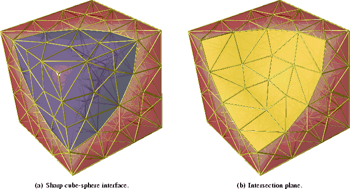
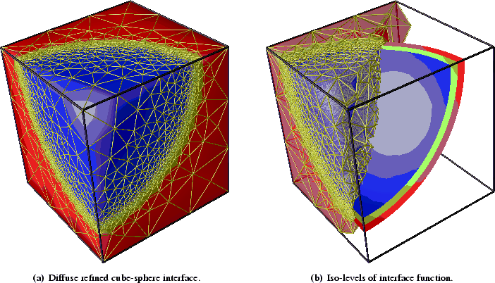
By the choice of a discrete interface representation on a three-dimensional tetrahedron based mesh, the interface itself is given by a set of triangles and their associated edges and points which are compulsory parts of the mesh elements. Figure 5.3 illustrates such a sharp interface for an introductive example. The interface is defined by the set of all yellow triangles depicted in Figure 5.3(b).

If the mesh is a conformal mesh, as defined in Section 2.1.8, then the interface must also be conformal. This means for our example, that the sphere and the cube can be glued together, and the union forms a conformal mesh again.

The advantage of sharp interfaces is their clear representation through geometric elements. For the three-dimensional tessellation based on unstructured tetrahedron meshes the interface can be defined by a set of triangles, edges, and points as depicted in Figure 5.3. Sharp interfaces are a good choice for static interfaces.

In the dynamic case a disproportional effort has to be undertaken to guarantee a conformal mesh for propagating interfaces, since the connectivity can change. The interface must be resolved over and over again for every time step. One very critical issue is to check, if interfaces merge together or pinch apart, because this causes special treatments and difficulties including, for example, determination of holes in the surface. One can imagine that the reorganization of such interfaces involves complicated remeshing procedures which are difficult to handle. This all gives motivation for another interface representation which is more suitable for dynamic interfaces, the group of so-called implicit interfaces.

5.2.2 Implicit Interface

The term implicit interface has its origin in the wide field of analytic geometry which is the area of mathematics that deals with the relation between geometry and mathematical expressions of coordinates of points in space. When applied to three-dimensional space, it is called solid analytic geometry [88,90]. The essential element of this mathematical field is a function which describes a geometric object.
For example, an explicit equation might express the $z$ -coordinate in terms of the $x$ and $y$ coordinates; that is $z=f(x,y)$ . Such a surface is called height field. Explicit representations show strong limitations in respect of the shape of the surface. It is not possible to describe closed surfaces with an explicit surface representation.

One approach is to use a parametric representation. For a two-dimensional surface embedded in three-dimensional space, this leads to $x=f_x(s,t)$ , $y=f_y(s,t)$ , and $z=f_z(s,t)$ . The other approach in which we are more focused is implicit: the coordinates are treated as functional arguments rather than functional values.

Usually surfaces are presented via, $F(x,y,z) = \vec{c}$ , where $\vec{c}$ is a point in $\mathbb{R}^n$ and $F$ maps $\mathbb{R}^n \mapsto \mathbb{R}^3$ . For most applications, $n$ is $1$ and $\vec{c}$ is a scalar. If $c$ is zero, we say that $f$ implicitly defines a locus called an implicit surface; that is, the set of points $\{\vec{p} \in \mathbb{R}^3 : f(\vec{p} ) = 0\}$ is a surface implicitly defined by $f$ . The function $f$ is called implicit surface function or a scalar field, a field function, or a potential function. The implicit surface is sometimes called the zero set of $f$ and may be written as $f^{-1}(0)$ or $Z(f)$ . The according iso-surface (also called a level set or level surface) is $\{\vec{p} \in \mathbb{R}^3 : f(\vec{p} ) = c\}$ , where $c$ is the iso-contour value of the surface [91,92].

For more sophisticated surfaces without analytical representation, we need to use a discretization. This means, $f$ can be seen as a pointwise sampled function according to the points of a three-dimensional mesh where each vertex holds a value of $f$ . To get a smooth representation of $f$ all over the three-dimensional domain, an interpolation scheme for function values between the sampling points is used.

In this work a linear basis function interpolation scheme was used which is very common in the field of finite element calculations as discussed in Section 3.1.3. The exact position of the interface is now determined by the chosen interpolation scheme and the mesh density, whereby the latter can be influenced by appropriate mesh adaptation techniques.

Figure 5.4: Implicit interface representation between the sphere and the cube. Due to the usage of linear interpolation between the mesh points, the interface defined by Equation (5.3) smears out. A cross cut through the mesh structure and level surfaces are plotted for iso-contour values $-0.98$ (blue), $0.00$ (green) , and $0.98$ (red) in the right picture.

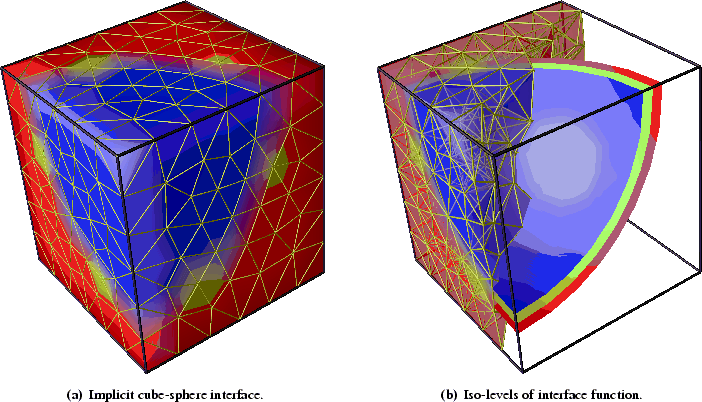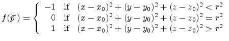
Back to the illustration example, Figure 5.4 shows the implicit interface representation between the sphere and the cube. A sphere with radius $r$ and center point $\vec{m}=(x_0,y_0,z_0)^T$ can be implicitly written as:

$$f_{sphere} = (x-x_0)^2 + (y-y_0)^2 + (z-z_0)^2 - r^2 = 0.$$ (5.2)

In this particular case the sphere-cube interface function with respect to (5.2) is defined similar to a Heaviside function [93]:

$$f(\vec{p} )=\left\{ \begin{array}{r l l} -1 & \text{if} & (x-x_... ... \ 1 & \text{if} & (x-x_0)^2 + (y-y_0)^2 + (z-z_0)^2 > r^2 \end{array} \right.$$ (5.3)

where for the example, $r$ was set to $75\%$ of the side length of the cube. The evaluation of the interface definition given by Equation (5.3) for every vertex of an existing mesh for the cube yields Figure 5.4(a), where the coloration mirrors the values of $f(\vec{p} )$ . A linear interpolation scheme was used for the evaluation of function points between the three-dimensional sampling points.

Due to the linear interpolation scheme and an unstructured tetrahedron based mesh the Heaviside function smears out and a wider interface region appears than initially defined by (5.3). Figure 5.4(b) shows level surfaces for the iso-contour values $-0.98$ (blue), $0.00$ (green), and $0.98$ (red).

Numerical interpolation produces an error in the estimation of $f$ . This can lead to perturbing or moving the interface away from its exact position. If these interface perturbations are small, their effects may be minor and a perturbed interface might be acceptable. In general, most numerical methods depend on the fact that their results are stable in the presence of small perturbations. If this is not true, then the problem under consideration is probably ill-posed and numerical methods should be used with extreme caution. These interface perturbation errors decrease as the number of sample points increases, implying that the exact answer could hypothetically be computed as the number of sample points is increased to infinity, which is the basis for most numerical methods [94].

It seems unlikely that any standard numerical approximation based on sampling will give a good approximation to a Heaviside like function. A wide range of smooth approximations of the Heaviside function are in use, which are commonly defined by limits. In the following three examples of such definitions are given, further definitions can be found e.g. in [95,96].

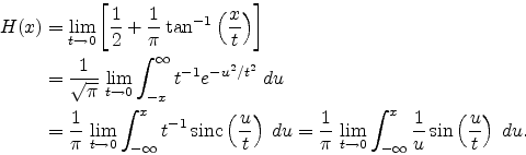$$\begin{split}H(x) &= \underset{t \rightarrow 0}{\lim} \left[ ... ... \frac{1}{u} \sin \left( \frac{u}{t} \right) du. \end{split}$$ (5.4)

For the simulation of void migration in interconnect lines, a special representation of an implicit interface function is used, where the interface width itself is varied. This interface is part of the following.

5.2.3 Diffuse Interface Model

A special kind of implicit interfaces is the so-called diffuse interface which is driven by the modeling of void migration and void growth due to bulk diffusion. This particular interface representation is mostly governed by the Cahn-Hilliard equation [97] where the void structure is described by an order parameter field, $\phi(\vec{x},t)$ that separates the interconnect line into a material phase and a void phase with a thin interface between them. The structure of the interface model equations in an unpassivated interconnect line can be written as

$$\frac{\partial \phi}{\partial t}= f_1(\mu,V,\varepsilon) \quad \mu=f_2(\varepsilon,\phi),$$ (5.5)

where $V$ is the electrical potential, $\mu$ denotes the chemical potential, and $\varepsilon$ is a parameter controlling the void-metal interface [98,99].

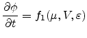
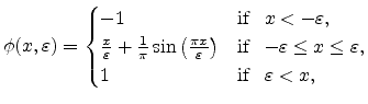
The used one-dimensional interface definition function in the value range from $-1$ to $1$ reads:

$$\phi(x,\varepsilon)= \begin{cases}-1& \text{if \; $x < - \varepsi... ...on \le x \le \varepsilon $}, \ 1& \text{if \; $\varepsilon < x $}, \end{cases}$$ (5.6)

where $\varepsilon$ determines the size of numerical smearing. In [94] a rule of thumb gives a value of $\varepsilon = 1.5 \Delta h$ for the tuning parameter on a uniform grid with a constant spacing of $\Delta h$ . This makes the interface width equal to three grid cells. Figure 5.5 shows a one-dimensional interface definition function, cf. Equation (5.6), with emphasis on different values for the tuning parameter  $\varepsilon$ .

Figure 5.5: Tunable one-dimensional interface definition function.

An increase of $\varepsilon$ causes a wider interface and increases numerical stability, but too flat transitions should also be avoided due to the loss of accuracy in the iso-level finding procedure. This problem is comparable with finding an intersection point of two straight line segments with a very small intersection angle [100]. Turning $\varepsilon$ close to zero gives a very sharp transition which defines a clear boarder but can lead to numerical instability in the face of spatial sampling.

One way to increase spatial resolution and therefore numerical accuracy is to use a finer mesh all over the domain. Driving this idea to an extreme yields an infinite number of mesh points with a maximum on possible numerical accuracy.
The drawback of course is also infinite high computational expenses on both, calculating time and memory usage. To bear down this problem a third form, a mixed form between fine and coarse mesh is used. Since the interface uses only a small part of the whole mesh domain, one can increase the spatial resolution only in a small area surrounding the interface itself, which yields the so-called refined diffuse interface.

5.2.4 Refined Diffuse Interface

Figure 5.6 shows the same interface as presented in Figure 5.4, but now with an isotropic refined interface belt. For the zoning of the refinement procedure the three-dimensional extension of the interface function definition as depicted in Equation (5.6) itself can be used.
The tuneable parameter $\varepsilon$ is now also responsible for the refinement procedure, i.e. that only elements within the $\varepsilon$ -environment $-\varepsilon \le x \le \varepsilon$ are used for refinement. In this example an isotropic recursive refinement approach as described in Section 2.2.3 was used only for elements within the refinement belt, which forms mostly isotropic elements. Elements outside the belt are untouched and, therefore, almost not involved in the refinement process.

Figure 5.6: Diffuse refined interface representation between the sphere and the cube. A refined region surrounds the interface with higher mesh density and, therefore, a higher numerical accuracy is reached. A cross cut through the mesh structure and level surfaces are plotted for iso-contour values $-0.98$  (blue), $0.00$  (green) , and $0.98$  (red) in the right picture.

Due to the nature of the recursive approach the spatial zoning is not always guaranteed and influences possibly also regions outside of the interface zone. Another disadvantage is also the necessity of tracing the interface in the case of a dynamic interface. After each time step the interface propagates and, therefore, the $\varepsilon$ -environment becomes also time dependent, i.e. the refinement procedure has to observe the interface. If the interface moves into new regions which are previously untouched, they have to be refined.

On the one hand side this tracking guarantees always a good resolution of the interface, on the other hand side it slows down the simulation, because only new points are added. Old ones which are run out of the interface zone remain still present.

Remediation of this matter is performed with the so-called hierarchical mesh refinement-coarsement scheme which is part of the next section.

5.2.5 Hierarchical Mesh Refinement-Coarsement Scheme

According to the demands of void movement simulation during electromigration also a mesh coarsening step has to be introduced. In analogy to the term ``refinement'', the coarsening procedure was named coarsement. The basic idea behind this coarsement strategy is that a previous refinement step is reversed. This procedure can be handled easily by introducing a hierarchical element structure as shown in Figure 5.7 and is therefore called hierarchical mesh refinement-coarsement scheme.

Figure 5.7: Data structure of a hierarchical refinement-coarsement scheme.

During transient simulation the position of the interface belt is detected after each timestamp and the mesh resolution is controlled. Too coarse elements are refined by recursive tetrahedral bisection. Regions which have been refined in a previous step and which are not covered by the void-metal interface any longer, are loaded into the coarsement module. Due to the properties of the hierarchical element data structure, the initial (before refinement) mesh constellation can be recovered easily.

It is in the nature of this approach that the initial mesh is always a subset of the current mesh and no coarser mesh than the initial one can be reached. This seems to be a handicap, however, the coarsest mesh is defined by the initial one and therefore the lowest spatial resolution is known, which controls the numerical error introduced by the starting mesh [101].