In the following three examples are presented which are carried out with the
VMC(Vienna Monte Carlo) simulator developed at
the Institute for Microelectronics. The very first version of VMC was
written in Fortran for stationary electron transport in polar semiconductors,
assuming analytical multi-valley band structures and bulk material [119]
generalized to covalent cubic semiconductors and semiconductor alloys. Over the
years this simulator has been extended to a full band, selfconsistent Monte
Carlo device simulator.
As described in the preamble of Section 6, any bounded volume of
silicon will contain a finite number of states. These energy values can be
derived from the number of energy levels in the isolated atoms. For the
determination of the properties of a semiconductor such as silicon it is
important to know the contributions from each occupied state and to sum them up.
The number of states is normally very large and so it is more convenient to sum
up over a range of states in
![]() -space. However, to do so, one needs to know the
density of states (DoS) in
-space. However, to do so, one needs to know the
density of states (DoS) in
![]() -space. A good introduction into calculating
the density of states is given in [114].
-space. A good introduction into calculating
the density of states is given in [114].
In the first example, the density of states for the conduction band of silicon
with
the typical parabolic and non-parabolic energy band approximations are compared
to the results found by a full band Monte Carlo approach with unstructured meshes for the
![]() -space. First a short overview on the calculation of the density of states is
given.
-space. First a short overview on the calculation of the density of states is
given.
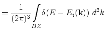
The density of states in the ![]() -th band, is defined by the following
formula [112,120]:
-th band, is defined by the following
formula [112,120]:
For the analytical non parabolic band structure Equation (6.17) evaluates to:
where
![]() is the density of states effective mass for the
is the density of states effective mass for the ![]() -th
valley, and
-th
valley, and
![]() denotes the band form function, cf. Equation (6.15):
denotes the band form function, cf. Equation (6.15):
For the full band case the density of states for one energy band reads:
where ![]() is the iso-surface for the given energy and band
in the irreducible wedge. Due to the symmetry of the band structure it is
sufficient to evaluate the integral only over the irreducible wedge and the factor
is the iso-surface for the given energy and band
in the irreducible wedge. Due to the symmetry of the band structure it is
sufficient to evaluate the integral only over the irreducible wedge and the factor
![]() accounts for all simular wedges in the Brillouin zone. Since the energy is
linearly interpolated, the velocity is constant and the iso-surface of energy is
plane within a tetrahedron. The contribution of the
accounts for all simular wedges in the Brillouin zone. Since the energy is
linearly interpolated, the velocity is constant and the iso-surface of energy is
plane within a tetrahedron. The contribution of the ![]() -th tetrahedron to the
density of states is
-th tetrahedron to the
density of states is
 |
(6.21) |
where
![]() is the area of the intersection of the
iso-surface of energy and the
is the area of the intersection of the
iso-surface of energy and the ![]() -th tetrahedron in the
-th tetrahedron in the ![]() -th energy band.
-th energy band.
In this example a direct comparison between a full band calculation for the
density of states and the analytical formula given in Equation (6.18)
is carried out. For the density of states the effective mass for an ellipsoidal
valley
![]() is given by
is given by
| (6.22) |
where the free electron rest mass is given by
![]() . The problem here is that different values for longitudinal
. The problem here is that different values for longitudinal ![]() ,
the transversal effective mass
,
the transversal effective mass ![]() , and for
, and for ![]() of silicon can be found in
the literature, e.g., [121,114,122]. In this work
of silicon can be found in
the literature, e.g., [121,114,122]. In this work
![]() and
and
![]() was used for the following calculations. For the band form function
in Equation (6.19)
was used for the following calculations. For the band form function
in Equation (6.19)
![]() was chosen.
was chosen.
In Figure 6.10(a) the density of states of the first three conduction bands
and the sum of them are plotted separately. It can be seen that the third
conduction band comes into play only at energies higher than
![]() . For transport calculations higher bands are of less importance and therefore
are frequently not taken into account.
. For transport calculations higher bands are of less importance and therefore
are frequently not taken into account.
Figure 6.10(b)
shows a comparison between the analytical parabolic and non-parabolic
approximations as discussed in Section 6.3 and
the density of states calculated by the full band approach. The parabolic model
is valid only for energies smaller than
![]() . Beyond this value
the parabolic model underestimates the density of states. The non-parabolic
approximation model overestimates the density of states and gives a more or
less feasible approximation for an energy up to
. Beyond this value
the parabolic model underestimates the density of states. The non-parabolic
approximation model overestimates the density of states and gives a more or
less feasible approximation for an energy up to
![]() . However,
for higher energies or more accurate simulations the full band Monte Carlo
method should be used.
. However,
for higher energies or more accurate simulations the full band Monte Carlo
method should be used.
![\begin{figure*}\setcounter{subfigure}{0}
\center
\mbox{\subfigure[Density of sta...
...roach.]
{\epsfig{figure =pics/diff.eps,width=0.48\textwidth}}}
\end{figure*}](img500.png) |
Two different meshing approaches are used to calculate the
average kinetic energy for different temperature values.
For the structured approach the mesh density is constant over the whole octant
of the first Brillouin zone, whereas for the unstructured approach the mesh density
is finer in particular regions of interest and therefore the mesh density
varies over the domain.
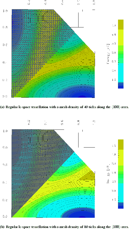
For the construction of the structured case a cubic grid based approach was
used, as described in Section 6.4.1.Further different grid
spacing is used to adjust the overall grid density. Figure 6.11
shows the used grid spacings. The coarser mesh features ![]() equally distributed cube ticks along the
equally distributed cube ticks along the
![]() -axes, where
every cube is divided into six tetrahedra as shown in the second row of
Figure 6.6. For the finer mesh, shown in Figure 6.11(b) a
grid spacing of
-axes, where
every cube is divided into six tetrahedra as shown in the second row of
Figure 6.6. For the finer mesh, shown in Figure 6.11(b) a
grid spacing of ![]() ticks along the
ticks along the
![]() -axes was chosen.
The same cubic grid representation was chosen for different conduction bands.
-axes was chosen.
The same cubic grid representation was chosen for different conduction bands.
 |
For the unstructured mesh of the first conduction band additional to the mesh
depicted in Figure 6.9(a) a finer mesh was used to see the
impact of the granularity of unstructured meshes. The second and third
conduction band was discretized with the meshes shown in
Figure 6.9(b) and Figure 6.9(c), respectively.
Table 6.1 gives an overview about the amount of points and
tetrahedra used for the spatial discretization of the first
octant of the Brillouin zone. The main distinction is focused on two meshing
approaches, namely the cubic grid approach, named structured, and the
pure unstructured mesh approach. Different overall mesh densities
are used in both areas, in the structured and the unstructured case. Additional for
the unstructured mesh representation of the first conduction band, a fine and
a coarse mesh is used. For the second and third band only one mesh is used,
see Figure 6.9(b) and Figure 6.9(c), respectively.
In the structured case the same granularity is used for all bands.
The particles of matter at ordinary temperatures can be considered to be in ceaseless, random motion. The average kinetic energy for these particles can be deduced from the classical Boltzmann distribution and gives for three-dimensional motion the theoretical formula [123]:
The electron gas in a semiconductor material deviates from Equation 6.23 as the parabolic band approximation does not hold. In the following a simulation has been carried out, where the zero field mean energy for electrons in undoped relaxed silicon with a full band structure for the first three conduction bands has been considered and compared with the theoretical value of the kinetic energy for parabolic bands given in (6.23).
![\includegraphics[width=0.6\textwidth,height=0.5\textwidth]{pics/emean3.eps}](img519.png)
|
Figure 6.12 shows that for temperatures below
![]() the
structured approach delivers results far above the theoretical value, so the
structured coarse mesh is useless even for room temperatures. The unstructured
approach converges for temperatures less than
the
structured approach delivers results far above the theoretical value, so the
structured coarse mesh is useless even for room temperatures. The unstructured
approach converges for temperatures less than
![]() against the theoretical value of
against the theoretical value of
![]() . For temperatures above room
temperature a difference of approximately
. For temperatures above room
temperature a difference of approximately ![]() can be observed which is due to
the non-parabolic property of the bands. The comparison between the fine and
the coarse
unstructured meshes gives rise to the deduction that the influence of the mesh
mostly depends on a good resolution of the low energy pockets of the first
conduction band, which is obviously clear for low temperatures, because under
such conditions all the electrons are found almost exclusively in the first
conduction band.
can be observed which is due to
the non-parabolic property of the bands. The comparison between the fine and
the coarse
unstructured meshes gives rise to the deduction that the influence of the mesh
mostly depends on a good resolution of the low energy pockets of the first
conduction band, which is obviously clear for low temperatures, because under
such conditions all the electrons are found almost exclusively in the first
conduction band.
In Section 6.5.2 an example was presented where almost all electrons
are found exclusively in the low energy pockets of the first conduction
band. In the following the electric field influence on the electron velocity is
calculated. In this scenario electrons gain higher energy values, which causes
a population of electrons in the whole Brillouin zone.
The particle motion within the Boltzmann transport equation picture consists
of consecutive scattering events and accelerations by external
forces [105,124]. In the following the electron velocity is calculated
from a Monte Carlo simulation under the influence of an
external electric field. For the
![]() -space discretization again different
meshes are compared, for a detailed overview see Table 6.1 in
Section 6.5.2.
-space discretization again different
meshes are compared, for a detailed overview see Table 6.1 in
Section 6.5.2.
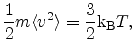
Figure 6.13 shows a comparison of simulation results for the
velocity as a function of the field for both structured and unstructured
tetrahedral meshes. As the curves for ![]() K and as well for
K and as well for ![]() K are grouped
very closed together above
K are grouped
very closed together above ![]() , it can be concluded that all meshes are
equally well suited. These results demonstrate that the
unstructured meshes perform very well in the high energy regimes, despite they
contain less mesh elements than the structured meshes.
, it can be concluded that all meshes are
equally well suited. These results demonstrate that the
unstructured meshes perform very well in the high energy regimes, despite they
contain less mesh elements than the structured meshes.
In order to get an impression of computational costs with emphasis on the CPU
time, in Table 6.2 an overview, with respect to different mesh
approaches is given. The CPU time is divided into the mesh data structure
build-up time, which is required only once at the beginning of the simulation and
two typical field point calculations, one in the low field regime at ![]() and a second one at
and a second one at ![]() . For every field point calculated the total
amount of scattering events was set to
. For every field point calculated the total
amount of scattering events was set to
![]() . For the calculations a
commercially obtainable Intel
. For the calculations a
commercially obtainable Intel![]() Pentium
Pentium![]() 4 CPU with
4 CPU with
![]() was used and the user processes CPU time was measured.
was used and the user processes CPU time was measured.
One can clearly see that the CPU time consumption is high for the structured meshes. The unstructured fine mesh demands approximately the same time as the coarse structured mesh, but one has to keep in mind, that the structured mesh fails completely for average kinetic energy at temperatures less than room temperature and the coarse unstructured mesh is still feasible.
![\includegraphics[width=0.64\textwidth,height=0.53\textwidth]{pics/highFieldComp3.eps}](img524.png)