In this section some well established definitions of
statistical terms are given. The following explanations are adapted
from [47], but can be found in any basic book which
deals with statistical mathematics.
Suppose there is a random population (or data set)
![]() , where
, where
| (A.1) |
and the mean of that population is given by
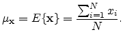 |
(A.2) |
For the standard deviation of a random variable
![]() we define:
we define:
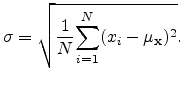 |
(A.3) |
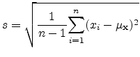
Finding the standard deviation of an entire population is in general
unrealistic. In most cases a sample standard deviation ![]() is used to
estimate a population standard deviation
is used to
estimate a population standard deviation
![]() . Given only a sample of
values
. Given only a sample of
values
![]() from some larger population
from some larger population
![]() with
with ![]() , the sample (or estimated) standard deviation is given by:
, the sample (or estimated) standard deviation is given by:
and the variance
![]() is simply the standard
deviation squared, which can be written as
is simply the standard
deviation squared, which can be written as
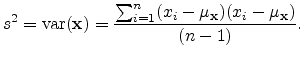 |
(A.5) |
The reason for this definition is that
![]() is an
unbiased estimator for the variance
is an
unbiased estimator for the variance
![]() of the underlying population
(see [125] for a detailed description). However, in the following
Equation (A.4) is used for calculating the standard deviation.
of the underlying population
(see [125] for a detailed description). However, in the following
Equation (A.4) is used for calculating the standard deviation.
Roughly speaking the variance gives a measure of the spread of data in a population. Standard deviation and variance operate only on one-dimensional data, which is very limiting, since many populations have more than one dimension.
For multi-dimensional data sets it is useful to define a measure in order to
find out, how much the dimension vary from the mean with respect to each other.
Covariance is such a measure and is defined for two data sets
![]() and
and
![]() via:
via:
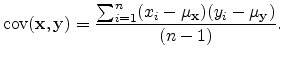 |
(A.6) |
It is straightforward to show that the covariance of two equal data sets form
the variance of the data set. Additionally the following characteristic holds
![]() since multiplication is commutative.
since multiplication is commutative.
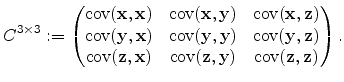
For ![]() -dimensional data sets it is possible to calculate
-dimensional data sets it is possible to calculate
 |
(A.7) |
different covariance values (without variance values, where
![]() ),
which can be written as matrix, the so-called
covariance matrix
),
which can be written as matrix, the so-called
covariance matrix
![]() defined by:
defined by:
where ![]() is the
is the ![]() dimension. For the following the dimension is set to
three, using the usual dimensions
dimension. For the following the dimension is set to
three, using the usual dimensions
![]() ,
,
![]() , and
, and
![]() , the covariance matrix reads
, the covariance matrix reads
 |
(A.9) |
This equation is known as the characteristic equation of
![]() , and the
left-hand side is known as the characteristic polynomial.
, and the
left-hand side is known as the characteristic polynomial.
PCA uses the eigenvalues and eigenvectors of the covariance matrix to form a
feature vector by ordering the eigenvalues from higher to lower. So the
eigenvector with the highest eigenvalues gives the component with highest
significance of the data set. If lower eigenvalues with their corresponding
eigenvectors are ignored, a reduction of the dimensionality can be
introduced. Based on these feature vectors a new data set is derived, where the
original data are expressed through the feature vectors.
Basically this is a transformation of the initial data set to express the data in terms of the patterns between them. This transformation is also known as Karhunen and Leove (KL) transform which was originally introduced as a series expansion for continuous random processes or for discrete random processes as Hotelling transform [126]. The following references are highly recommended for readers who are interested in PCA more deeply. A good introduction can be found in [47], a more general advise is given in the book of Jolliffe [46], and for application of PCA to computer vision [127] can be proposed.