B.2 Least Squares Approximation

The following is a summarization of articles in [62,63], a good introduction on this topic can also be found in [134] and [135]. A modern description for curves and surface fits is given in [61].

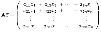
Linear systems can be represented in matrix form as the matrix equation $\mathbf{A}\vec{x}=\vec{b}$ , where

$$\mathbf{A}\vec{x}= \left( \begin{array}{cccc} a_{11}x_{1}\:\;+ &\... ...}x_{2}\:\;+ &\!\!\!\!\!\cdots\:\;+ &\!\!\!\!\!a_{mn}x_{n}\ \end{array} \right)$$ (B.4)

and $\vec{b}=(b_{1},b_{2},\cdots,b_{m})^T$ . If the linear system holds more equations $m$ than the number variables $n$ , no exact solution may be found.

One possible way is to find an approximate solution of the linear system given by Equation (B.4) by means of a least squares approximation.

In mathematical terms,

$$\mathbf{A}\vec{x} \approx \vec{b}$$ (B.5)

where $\mathbf{A}$ is an $m$ -by-$n$ matrix (with $m > n$ ) and $\vec{x}$ and $\vec{b}$ are $n$ -, respectively $m$ -dimensional column vectors. More precisely, the least squares approximation has to minimize the Euclidean norm of the squared residual $\mathbf{A}\vec{x}-\vec{b}$ , that is, the quantity

$$\Vert\mathbf{A}\vec{x}-\vec{b} \Vert^2 = \left([\mathbf{A}x]_1-... ... +\left([\mathbf{A}x]_2-b_2\right)^2 +\dots+ \left([\mathbf{A}x]_n-b_n\right)^2$$ (B.6)

where $[\mathbf{A}x]_i$ denotes the $i$ -th component of the vector $\mathbf{A}\vec{x}$ . Hence the name least squares. Using the fact that the squared norm of a vector $\vec{v}$ is $\vec{v} ^T\vec{v}$ , (B.6) can be rewritten as

$$(\mathbf{A}\vec{x}-\vec{b} )^T(\mathbf{A}\vec{x}-\vec{b} ) = ... ... ^T \mathbf{A}\vec{x} - (\mathbf{A}\vec{x} )^T\vec{b} + \vec{b} ^T \vec{b}.$$ (B.7)

The two mixed terms are identical. The minimum is found at the zero of the derivative with respect to $\vec{x}$ ,

$$2\mathbf{A}^T\mathbf{A}\vec{x} - 2\mathbf{A}^T\vec{b} = 0.$$ (B.8)

Therefore, the minimizing vector $\vec{x}$ is a solution of the normal equation

$$\mathbf{A}^T\mathbf{A}x=\mathbf{A}^{T}b,$$ (B.9)

where $\mathbf{A}^T$ denotes the transposed form of $\mathbf{A}$ , and equation (B.9) corresponds to a system of linear equations. The matrix $\mathbf{A}^T\mathbf{A}$ on the left hand side is a square matrix, which is invertible, if $\mathbf{A}$ has full column rank (that is, if the rank of $\mathbf{A}$ is $n$ ). In that case, the solution of the system of linear equations is unique and given by

$$x= (\mathbf{A}^T\mathbf{A})^{-1} \mathbf{A}^{T}b.$$ (B.10)

The matrix $(\mathbf{A}^T\mathbf{A})^{-1} \mathbf{A}^{T}$ is called a pseudo inverse of $\mathbf{A}$ , since the true inverse of $\mathbf{A}$ (that is $\mathbf{A}^{-1}$ ) does not exist as $\mathbf{A}$ is not a square matrix ($m \neq n$ ).