« Previous Up Next »Contents
Previous: 6 Summary and Outlook Top: Home Next: B Vacancies in a Crystal Lattice

A The Asymptotic Limit of the Phase Field Model

In this chapter the behavior of the phase field model in its asymptotic limit is discussed, as described by Bhate et al. [9]. The analysis shows that in the limit of an infinitely thin interface the phase field model equations converge to the equations of the sharp interface model. The interface thickness, described in Section 3.6, is controlled by the parameter $\epsilon _{\mathrm {p}\mathrm {f}}$ and, therefore, the asymptotic limit to an infinitely thin interface is accomplished by driving this parameter against zero [38].

For an easier handling the governing equations are rewritten in a dimensionless form [9]:

$(1.1–A.2) \{begin}{gather} \displaystyle \frac {\partial \phi }{\partial \tilde {t}}=\frac {2}{\tilde {\epsilon }\pi }\tilde {\nabla } \Bigl (\tilde {D}_{\mathrm {s}}\Bigl (\tilde {\nabla }\tilde {\mu }-\chi \tilde {\nabla }\tilde {\phi }_{\mathrm {E}}\Bigr )\Bigr ) -\displaystyle \frac {4}{\tilde {\epsilon }\pi }\tilde {J}_{\mathrm {n}\mathrm {v}}, \mathref {(A.1)} \\ =\displaystyle \frac {2}{\tilde {\epsilon }\pi }\tilde {\nabla } \Bigl (\tilde {D}_{\mathrm {s}}\tilde {\nabla }\tilde {\mu }^{*}\Bigr ) -\displaystyle \frac {4}{\tilde {\epsilon }\pi }\tilde {J}_{\mathrm {n}\mathrm {v}}, \mathref {(A.2)} \{end}{gather}$

where in $\tilde {\nabla }\tilde {\mu }^{*}$ both the gradient of the chemical potential $\tilde {\nabla }\tilde {\mu }$ and the therm due to the electric field $-\chi \tilde {\nabla }\tilde {\phi }_{\mathrm {E}}$ are added and

$(A.3) \{begin}{gather} \displaystyle \tilde {\mu }=\frac {4}{\tilde {\epsilon }\pi } \Bigl (f’(\phi )-\tilde {\epsilon }^{2}\tilde {\triangle }\phi \Bigr ) +2\displaystyle \Lambda \frac {\partial \tilde {W}}{\partial \phi }, \mathref {(A.3)} \{end}{gather}$

where the connection between the dimensionless quantities and the quantities with units

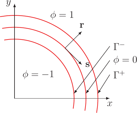
Figure A.1.: Figure A.1.: Illustration of the partitioning of the void metal region into interface, void, and metal domains for the inner expansion [9].

are given by

$(1.4–A.10) \{begin}{gather} \epsilon _{\mathrm {p}\mathrm {f}}=\tilde {\epsilon }a, \mathref {(A.4)} \\ x=\tilde {x}a, {\mathref {(A.5)}} \\ t=\tilde {t}\frac {a^{4}}{\Omega \gamma _{\mathrm {s}}D_{\mathrm {s}}’}, {\mathref {(A.6)}} \\ \phi _{\mathrm {E}}=\tilde {\phi }_{\mathrm {E}}E^{*}a, {\mathref {(A.7)}} \\ W=\tilde {W}W^{*}, {\mathref {(A.8)}} \\ J_{\mathrm {n}\mathrm {v}}=\displaystyle \tilde {J}_{\mathrm {n}\mathrm {v}}\frac {\Omega \gamma _{\mathrm {s}}D_{\mathrm {s}}}{a^{3}}, {\mathref {(A.9)}} \\ \displaystyle \mu =\tilde {\mu }\frac {\Omega \gamma _{\mathrm {s}}}{a}. \mathref {(A.10)} \{end}{gather}$

There $a$ is a characteristic length, $E^{*}$ is a characteristic electric field strength, and $W^{*}$ is a characteristic strain energy. Furthermore, $\Omega$ is the volume of an atom in the lattice, $\gamma _{\mathrm {s}}$ is the surface energy of the metal/void interface, and $D_{\mathrm {s}}$ is the diffusion coefficient at the metal surface.

In the further discussion the tilde sign above the dimensionless values will be omitted for easier reading. If a distinction is needed, it will be explicitly pointed out. The parameters in (A.1) and (A.3) are given by

$(1.11–A.12) \{begin}{gather} \displaystyle \chi =\frac {eZ^{*}E^{*}a^{2}}{\Omega \gamma _{\mathrm {s}}}, \mathref {(A.11)} \\ \displaystyle \Lambda =\frac {W^{*}a}{\gamma _{\mathrm {s}}}, \mathref {(A.12)} \{end}{gather}$

where the quantities $\chi$ and $\Lambda$ are dimensionless numbers characteristic for the formulated problem.

For the derivation a local coordinate system is chosen, as already used for the sharp interface model. This coordinate system is extended to the region of the diffuse interface and splits up the simulation domain into three regions. The regions are the metal region, the void region, and the interface region separating the two former (cf. Figure A.1).

The derivations for the asymptotic limit is carried out in two steps. First the formulas are transformed into the local coordinate system. This step is followed by the introduction of the Taylor expansion in $\epsilon$ of the functions and a splitting of the equations in terms of $\epsilon$ -orders.

For the local coordinate system, some definitions are required regarding the calculation of the normal vector $\mathbf {n}$

$(A.13) \{begin}{gather} \mathbf {n}=-\nabla _{x}r \mathref {(A.13)} \{end}{gather}$

and the curvature $\kappa$ for the $\phi =0$ contour.

$(A.14) \{begin}{gather} \kappa =\triangle _{x}r \mathref {(A.14)} \{end}{gather}$

The subscript $x$ is used for the common differential operators. Furthermore, the normal velocity of the interface is expressed by the time derivative of the $\phi = 0$ contour (interface)

$(A.15) \{begin}{gather} v_{n}=\displaystyle \frac {\partial r}{\partial t}, \mathrm {\mathref {(A.15)}} \{end}{gather}$

and the $r$ -coordinate of the local coordinate system is normalized as

$(A.16) \{begin}{gather} \displaystyle \rho =\frac {r}{\epsilon }. \mathref {(A.16)} \{end}{gather}$

As the asymptotic expansion is carried out in the local coordinate system all functions have to be expressed in this coordinate system as well:

$(A.17) \{begin}{gather} \psi (\mathbf {x})=\Psi (r(\mathbf {x}),\ s(\mathbf {x})) \mathref {(A.17)} \{end}{gather}$

For the time derivative the chain rule gives

$(A.18) \{begin}{gather} \displaystyle \frac {\partial \psi }{\partial t}=\Psi _{t}+\Psi _{s}\frac {\partial s}{\partial t}+\Psi _{r}\frac {\partial r}{\partial t} , \mathref {(A.18)} \{end}{gather}$

where the indices after the comma stand for the derivative

$(A.19) \{begin}{gather} \displaystyle \Psi _{k}=\frac {\partial \Psi }{\partial k}. \mathref {(A.19)} \{end}{gather}$

By again employing the chain rule the $\nabla _{x}$ operator can be expressed in the new coordinate system by

$(A.20) \{begin}{gather} \nabla _{x}\psi =\Psi _{s}\nabla _{x}s+\Psi _{r}\nabla _{x}r. {\mathref {(A.20)}} \{end}{gather}$

The last needed differential operator is the Laplace operator given by

$(A.21) \{begin}{gather} \triangle _{x}\psi =\triangle _{s}\Psi +\Psi _{r}\triangle _{x}r+\Psi _{rr}|\nabla r|^{2} \mathref {(A.21)} \{end}{gather}$

in the new coordinate system, where the first term, containing only functions $\Psi$ differentiated with respect to $s$ , is defined by

$(A.22) \{begin}{gather} \triangle _{s}\Psi =\Psi _{ss}|\nabla s|^{2}+\Psi _{s}\triangle _{x}s. \mathref {(A. 22)} \{end}{gather}$

The boundary conditions for the $\Gamma ^{-}$ and $\Gamma ^{+}$ contour for the phase field function (cf. Figure A.1) are given by

$(A.23) \{begin}{gather} \displaystyle \lim _{x\rightarrow \Gamma ^{\pm }}\phi =\pm 1 {\mathref {(A.23)}} \{end}{gather}$

as there the pure metal or the pure void starts and

$(A.24) \{begin}{gather} \displaystyle \lim _{x\rightarrow \Gamma ^{\pm }} \frac {\partial \phi }{\partial \mathbf {n}} =0, {\mathref {(A.24)}} \{end}{gather}$

as the phase field function has to be a smooth function everywhere and, therefore, also at the boundary contours between the metal and the interface and between the void and the interface. The flux at the interface has to be limited to the interface leading to a third boundary condition of zero flux from the interface into the metal or the void given by

$(A.25) \{begin}{gather} \displaystyle \lim _{x\rightarrow \Gamma ^{\pm }} \Bigl (\displaystyle \frac {2D_{\mathrm {s}}}{\epsilon \pi }(\nabla \mu -\chi \nabla \varphi )\Bigr ) =0. {\mathref {(A.25)}} \{end}{gather}$

The inner expansion of the order parameter and the chemical potential, where the EM therm is included, is the Taylor expansion with respect to the interface thickness controlling parameter $\epsilon .$

$(1.26–A.28) \{begin}{gather} \phi =\phi _{0}+\epsilon \phi _{1}+\epsilon ^{2}\phi _{2}+\mathcal {O}(\epsilon ^{3}) \mathref {(A.26)} \\ \mu =\mu _{0}+\epsilon \mu _{1}+\epsilon ^{2}\mu _{2}+\mathcal {O}(\epsilon ^{3}) \mathref {(A.27)} \\ \mu ^{*}=\mu _{0}^{*}+\epsilon \mu _{1}^{*}+\epsilon ^{2}\mu _{2}^{*}+\mathcal {O}(\epsilon ^{3}) \mathref {(A. 28)} \{end}{gather}$

The constant multipliers $\displaystyle \frac {1}{n!}$ from the Taylor expansion are absorbed into the functions $\phi _{n}, \mu _{n}$ and $\mu _{n}^{*}$ . First the differential operators (A.18)-(A.21) for functions in the local coordinate system in (A.1) are employed, resulting in

$(A.29) \{begin}{gather} \displaystyle \frac {\partial \phi }{\partial t}=\phi _{t}+ \underbrace {\phi _{s}}_{=0} \displaystyle \frac {\partial s}{\partial t}+\phi _{r}\frac {\partial r}{\partial t} {\mathref {(A.29)}} \\ =\nabla \cdot \Bigl (\frac {2D_{\mathrm {s}}}{\epsilon \pi }\nabla \mu ^{*}\Bigr )\ -\frac {4}{\epsilon \pi }J_{\mathrm {n}\mathrm {v}} =\frac {2}{\epsilon \pi }\nabla D_{\mathrm {s}}\ \nabla \mu ^{*}+\frac {2}{\epsilon \pi }D_{\mathrm {s}}\triangle \mu ^{*}-\frac {4}{\epsilon \pi }J_{\mathrm {n}\mathrm {v}}\notag \\ =\frac {2}{\epsilon \pi }(\frac {\partial D_{\mathrm {s}}}{\partial \phi } \underbrace {\phi _{,s}}_{=0} \nabla _{x}s +\frac {\partial D_{\mathrm {s}}}{\partial \phi }\phi _{,r}\nabla _{x}r)\ (\mu _{,s}^{*}\nabla _{x}s+\mu _{,r}^{*}\nabla _{x}r)+\frac {2}{\epsilon \pi }D_{\mathrm {s}}\triangle \mu ^{*}-\frac {4}{\epsilon \pi }J_{\mathrm {n}\mathrm {v}}\notag \{end}{gather}$

$=\frac {2}{\epsilon \pi }(\frac {\partial D_{\mathrm {s}}}{\partial \phi }\phi _{r}\mu _{r}^{*})+\frac {2}{\epsilon \pi }D_{\mathrm {s}}(\triangle _{s}\mu ^{*}+\mu _{r}^{*}\triangle _{x}r+\mu _{rr}^{*})-\frac {4}{\epsilon \pi }J_{\mathrm {n}\mathrm {v}},$

where the derivatives of the phase field function with respect to the tangential direction are zero as in this direction the phase field function is constant (zero). Furthermore, $\nabla r$ and $\nabla s$ are orthogonal to each other and due to the normalization of $\mathrm {n}$ , the inner product of $\nabla r$ with itself is equal to one. Using $\displaystyle \frac {\partial }{\partial r} = \displaystyle \frac {1}{\epsilon }\frac {\partial }{\partial \rho }$ (e.g. $\mu _{,r}^{*}= \displaystyle \frac {\mu _{,\rho }^{*}}{\epsilon }$ ), derived from (A.16), results in

$(A.30) \{begin}{gather} \displaystyle \epsilon ^{2}\frac {\pi }{2}\phi _{t}+\epsilon \frac {\pi }{2}\phi _{\rho }\frac {\partial r}{\partial t}=\frac {1}{\epsilon }\frac {\partial D_{\mathrm {s}}}{\partial \phi }\phi _{\rho }\mu _{\rho }^{*}+\epsilon D_{s}\triangle _{s}\mu ^{*}+D_{s}\mu _{\rho }^{*}\kappa +\frac {1}{\epsilon }D_{s}\mu _{\rho \rho }^{*}-2J_{\mathrm {n}\mathrm {v}}. {\mathref {(A.30)}} \{end}{gather}$

Inserting the inner expansions (A.26) and (A.28) defined above and taking only terms to the first order in $\epsilon$ into account leads to the equation

$(A.31) \{begin}{gather} \epsilon \frac {\pi }{2}\phi _{0,\rho }\frac {\partial r}{\partial t}+\mathcal {O}(\epsilon ^{2})= \overbrace { \frac {1}{\epsilon }\frac {\partial D_{\mathrm {s}}}{\partial \phi }\phi _{0,\rho }\mu _{0,\rho }^{*}+ \frac {\partial D_{\mathrm {s}}}{\partial \phi }\phi _{0,\rho }\mu _{1,\rho }^{*}+\epsilon \frac {\partial D_{\mathrm {s}}}{\partial \phi }\phi _{0,\rho }\mu _{2,\rho }^{*}+\mathcal {O}(\epsilon ^{2})}^ {\frac {1}{\epsilon }\frac {\partial D_{\mathrm {s}}}{\partial \phi }\phi _{,\rho }\mu _{,\rho }^{*}}+\notag \\ \overbrace {\epsilon D_{\mathrm {s}}\triangle _{s}\mu _{0}^{*}+\mathcal {O}(\epsilon ^{2})}^ {\epsilon D_{\mathrm {s}}\triangle _{s}\mu ^{*}}+ \overbrace {D_{\mathrm {s}}\mu _{0,\rho }^{*}\kappa +\epsilon D_{\mathrm {s}}\mu _{1,\rho }^{*}\kappa +\mathcal {O}(\epsilon ^{2})}^ {D_{\mathrm {s}}\mu _{,\rho }^{*}\kappa }+\notag \\ \overbrace {\frac {1}{\epsilon }D_{\mathrm {s}}\mu _{0,\rho \rho }^{*}+D_{\mathrm {s}}\mu _{1,\rho \rho }^{*}+\epsilon D_{\mathrm {s}}\mu _{2,\rho \rho }^{*}+\mathcal {O}(\epsilon ^{2})} ^{\frac {1}{\epsilon }D_{\mathrm {s}}\mu _{,\rho \rho }^{*}} -2J_{\mathrm {n}\mathrm {v}}. \mathref {(A.31)} \{end}{gather}$

Reordering the equation by collecting the terms with the same order of $\epsilon$ and leaving away the terms of the second order leads to the equation

$\displaystyle \epsilon \frac {\pi }{2}\phi _{0,\rho }\frac {\partial r}{\partial t}=\frac {1}{\epsilon }\Bigl (\displaystyle \frac {\partial D_{\mathrm {s}}}{\partial \phi }\phi _{0,\rho }\mu _{0,\rho }^{*}+D_{\mathrm {s}}\mu _{0,\rho \rho }^{*}\Bigr ) + \Bigl (D_{\mathrm {s}}\displaystyle \mu _{0,\rho }^{*}\kappa +\frac {\partial D_{\mathrm {s}}}{\partial \phi }\phi _{0,\rho }\mu _{1,\rho }^{*}+D_{\mathrm {s}}\mu _{1,\rho \rho }^{*}\Bigr )$

$(A.32) \{begin}{gather} +\displaystyle \epsilon \Bigl (D_{\mathrm {s}}\triangle _{s}\mu _{0}^{*}+D_{\mathrm {s}}\mu _{1,\rho }^{*}\kappa +\frac {\partial D_{\mathrm {s}}}{\partial \phi }\phi _{0,\rho }\mu _{2,\rho }^{*}+D_{\mathrm {s}}\mu _{2,\rho \rho }^{*}-2J_{\mathrm {n}\mathrm {v}}\Bigr ) \{end}{gather}$

and the different orders of $\epsilon$ can be handled separately giving the following set of equations:

$(1.33–A.35) \{begin}{gather} \mathcal {O}(\epsilon ^{-1}):\quad 0=\overbrace {\displaystyle \frac {\partial D_{\mathrm {s}}}{\partial \phi }\phi _{0,\rho }\mu _{0,\rho }^{*}+D_{\mathrm {s}}\mu _{0,\rho \rho }^{*}}^{(D_s \mu _{0,\rho }^*)_{,\rho }=0} {\mathref {(A.33)}}\\ \mathcal {O}(\epsilon ^{0}):\quad 0=D_{\mathrm {s}}\displaystyle \overbrace {\mu _{0,\rho }^{*}}^{=0}\kappa +\overbrace {\frac {\partial D_{\mathrm {s}}}{\partial \phi }\phi _{0,\rho }\mu _{1,\rho }^{*}+D_{\mathrm {s}}\mu _{1,\rho \rho }^{*}}^{(D_s \mu _{1,\rho }^*)_{,\rho }=0} {\mathref {(A.34)}} \\ \mathcal {O}(\epsilon ^{1}) : \displaystyle \frac {\pi }{2}\phi _{0,\rho }\frac {\partial r}{\partial t}=D_{\mathrm {s}}\triangle _{s}\mu _{0}^{*}+D_{\mathrm {s}}\mu _{1,\rho }^{*}\kappa +\frac {\partial D_{\mathrm {s}}}{\partial \phi }\phi _{0,\rho }\mu _{2,\rho }^{*}+D_{\mathrm {s}}\mu _{2,\rho \rho }^{*}-2J_{\mathrm {n}\mathrm {v}} {\mathref {(A.35)}} \{end}{gather}$

The first over-brace in (A.33) shows that the term $D_{s}\mu _{0,\rho }^{*}$ is constant in $\rho$ . With the definition of the diffusion coefficient

$(A.36) \{begin}{gather} D_{\mathrm {s}}(\phi )= \left \{\begin {array}{l} 1\ \mathrm {i}\mathrm {f}\ |\phi |\ <\ 1,\\ 0\ \mathrm {o}\mathrm {t}\mathrm {h}\mathrm {e}\mathrm {r}\mathrm {w}\mathrm {i}\mathrm {s}\mathrm {e}\ ’ \end {array}\right . {\mathref {(A.36)}} \{end}{gather}$

it can be concluded that

$(A.37) \{begin}{gather} \mu _{0}^{*}=F(s,t) \mathref {(A.37)} \{end}{gather}$

and the first over-brace in (A.34) is zero as $\mu _{0}^{*}$ is independent of $\rho$ and the second over-brace in (A.34) can be handled like the first over-brace in (A.33).

$(A.38) \{begin}{gather} \mu _{1}^{*}=G(s,t) {\mathref {(A.38)}} \{end}{gather}$

Applying the same procedure of the transformation into the local coordinate system and applying the Taylor expansion to the chemical potential results in the equation

$\displaystyle \frac {\pi }{4}(\mu _{0}+\epsilon \mu _{1}+\mathcal {O}(\epsilon ^{2}))=\frac {1}{\epsilon }(-\phi _{0,\rho \rho }+f’(\phi _{0}))$

$(A.39) \{begin}{gather} +\Bigl (-\displaystyle \phi _{0,\rho }\kappa -\phi _{1,\rho \rho }+f”(\phi _{0})\phi _{1}+\frac {\pi }{2}\Lambda \frac {\partial W_{0}}{\partial \phi _{0}}\Bigr ) +\mathcal {O}(\epsilon ), {\mathref {(A.39)}} \{end}{gather}$

and a separation of the equation into a set of equations ordered by the order in $\epsilon$ gives

$(1.40–A.41) \{begin}{gather} \mathcal {O}(\epsilon ^{-1}):\quad 0=-\phi _{0,\rho \rho }+\overbrace {f’(\phi _{0})}^{-\phi _{0}} {\mathref {(A.40)}} \\ \mathcal {O}(\epsilon ^{0}):\quad \displaystyle \frac {\pi }{4}\mu _{0}=-\phi _{0,\rho }\kappa -\phi _{1,\rho \rho }+f”(\phi _{0})\phi _{1}+\frac {\pi }{2}\Lambda \frac {\partial W_{0}}{\partial \phi _{0}}, {\mathref {(A.41)}} \{end}{gather}$

where the double obstacle function defined in Section 3.6 was used for the bulk free energy defined by

$(A.42) \{begin}{gather} f(\phi )= \left \{\begin {array}{ll} \frac {1}{2}(1-\phi ^{2}) & \mathrm {i}\mathrm {f}\ |\phi |\ <\ 1,\\ \infty & \mathrm {o}\mathrm {t}\mathrm {h}\mathrm {e}\mathrm {r}\mathrm {w}\mathrm {i}\mathrm {s}\mathrm {e} \end {array}\right . {\mathref {(A.42)}} \{end}{gather}$

Setting the term of the order $\displaystyle \frac {1}{\epsilon }$ equal zero leads to the differential equation

$(A.43) \{begin}{gather} \phi _{0,\rho \rho }+\phi _{0}=0 {\mathref {(A.43)}} \{end}{gather}$

with the solutions

$(A.44) \{begin}{gather} \phi _{0}=A\sin (\rho )+B\cos (\rho ), {\mathref {(A.44)}} \{end}{gather}$

where, due to the boundary conditions (A.23) and (A.24), $A$ equals one and $B$ equals zero and the thickness of the interface in the $\rho$ coordinate is $\pi$ . Taking the terms of the zeroth order of $\epsilon$ of (A.39) and rearranging them leads to

$(A.45) \{begin}{gather} \displaystyle \phi _{1,\rho \rho }-f”(\phi _{0})\phi _{1}=-\frac {\pi }{4}\mu _{0}-\phi _{0,\rho }\kappa +\frac {\pi }{2}\Lambda \frac {\partial W_{0}}{\partial \phi _{0}}=R, {\mathref {(A.45)}} \{end}{gather}$

where $R$ is not a function of $\phi _{1}$ . This equation has the same structure as the derivative of (A.43) with respect to $\rho$ . Therefore only the trivial solution can meet the boundary conditions given by (A.24) and

$(A.46) \{begin}{gather} \phi _{1} \left (\displaystyle \pm \frac {\pi }{2},s,t\right ) =0. {\mathref {(A.46)}} \{end}{gather}$

Integrating (A.45) in $\rho$ direction over the whole interface region results in

$(A.47) \begin{equation} \includegraphics [width=97.20\mymm ,height=24.72\mymm ]{page_105_images/image001} {\mathref {(A.47)}} \end{equation}$

where the under-braces give the results of the integrals. With the assumption of zero elastic strain energy in the void this leads to

$(A.48) \{begin}{gather} \mu _{0}=-\kappa +\Lambda W_{0}. {\mathref {(A.48)}} \{end}{gather}$

This is the same equation as (3.47) and shows that the chemical potential in the asymptotic limit converges to the sharp interface model. Coming back to (A.32), taking the terms of first order in $\epsilon$ , and again integrating over the interface in $\rho$ gives

$(A.49) \{begin}{gather} \displaystyle \frac {\pi }{2}\overbrace {\frac {\partial r}{\partial t}}^{v_n} \overbrace {\int \limits _{\Gamma +}^{\Gamma -}\phi _{0,\rho }\mathrm {d}\rho }^2 =D_{\mathrm {s}} \triangle _{s}\mu _{0}^{*} \overbrace {\int \limits _{\Gamma +}^{\Gamma -}\mathrm {d}\rho }^\pi +\nonumber \\\int \limits _{\Gamma +}^{\Gamma -}D_{\mathrm {s}}\overbrace {\mu _{1,\rho }^{*}}^0 \kappa \mathrm {d}\rho +\int _{\Gamma ^-}^{\Gamma ^+}\underbrace {\frac {\partial D_s}{\partial \phi }\phi _{0,\rho }\mu ^*_{2,\rho }+D_s\mu ^*_{2,\rho \rho }}_{(D_{\mathrm {s}}\mu _{2,\rho }^{*})_{\rho }=0}d\rho -\int \limits _{\Gamma +}^{\Gamma -}2J_{nv}d\rho , {\mathref {(A.49)}} \{end}{gather}$

where for the third term on the right hand side the zero flux condition was employed, resulting in the equation for the normal velocity of the sharp interface model

$(A.50) \{begin}{gather} v_{n}=\triangle _{s}\mu _{0}^{*}-\hat {D}(\mu _{\mathrm {b}\mathrm {v}}-\mu _{\mathrm {s}\mathrm {v}}) {\mathref {(A.50)}} \\ =\triangle _{s}\mu _{0}-\chi \triangle _{s}\phi _{\mathrm {E}}-\hat {D}(\mu _{\mathrm {b}\mathrm {v}}-\mu _{\mathrm {s}\mathrm {v}})\ .\notag \{end}{gather}$

These evaluations show that the phase field model for $\epsilon _{\mathrm {p}\mathrm {f}}$ going to zero converges to the sharp interface model and can therefore be used for the simulations of voids as long as $\epsilon _{\mathrm {p}\mathrm {f}}$ is chosen carefully. The upper limit is in the order of the smallest curvature occurring at the surface of the voids. The lower limit is given by the meshing resolution. From one side of the boundary region to the other a minimum of five meshing elements is needed to guarantee the stability of the FEM simulation, as was found by empirical studies.

« Previous Up Next »Contents
Previous: 6 Summary and Outlook Top: Home Next: B Vacancies in a Crystal Lattice