4.1 Diffusion and Green's Functions

The simple linear diffusion differential equation reads

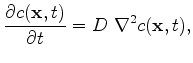$$\frac{\partial c({\mathrm{\bf x}},t)}{\partial t} = D \; \nabla^2 c({\mathrm{\bf x}},t),$$ (4.1)

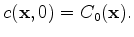
where $c$ denotes the time and space dependent concentration, with a constant diffusion coefficient $D$ and the initial condition

$$c({\mathrm{\bf x}},0)=C_{0}({\mathrm{\bf x}}).$$ (4.2)

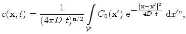
With the theory of Green's Functions the solution $c({\mathrm{\bf x}},t)$ of this differential equation problem for one, two, and three dimensions is obtained as

$$c({\mathrm{\bf x}},t)=\frac{1}{(4 \pi D t)^{\mathrm{n}/2}} \in... ...-{\mathrm{\bf x}}'\vert^2}{\scriptstyle 4 D t}} \;\mathrm{d}x'^{\mathrm{n}},$$ (4.3)

where $\mathrm{n}$ is the dimensionality of the problem.

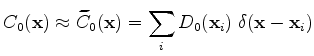
The discretization of this problem is performed by the following method: After the simulation domain is meshed and the Delaunay boxes are determined, the initial distribution $c({\mathrm{\bf x}},0)$ is discretized on the grid points by Dirac functions

$$C_0({\mathrm{\bf x}}) \approx \widetilde{C}_0({\mathrm{\bf x}}) = \sum_{i} D_0({\mathrm{\bf x}}_i) \;\delta({\mathrm{\bf x}} - {\mathrm{\bf x}}_i)$$ (4.4)

with

$$D_0({\mathrm{\bf x}}_i)=\int\limits_{\mathcal{V}_i} C_0 ({\mathrm{\bf x}}) \;\mathrm{d}v.$$ (4.5)

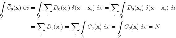
The preservation of the total implantation dose in the simulation domain

$$\begin{gather*}\begin{split}\int\limits_\mathcal{V} \widetilde{C}_0 ({\mathrm{\b... ...imits_\mathcal{V} C_0({\mathrm{\bf x}}) \;\mathrm{d}v= N\end{split}\end{gather*}$$ (4.6)

is guaranteed by the discretization of the initial distribution.

As a consequence by applying (4.3), the approximated transient concentration distribution can be evaluated by

$$\begin{gather*}\begin{split}c({\mathrm{\bf x}},t) \approx \widetilde{c}({\mathrm... ...x}}-{\mathrm{\bf x}}_i'\vert^2}{\scriptstyle 4 D t}}.\end{split}\end{gather*}$$ (4.7)

The total dose in the whole space $\mathcal{R}$

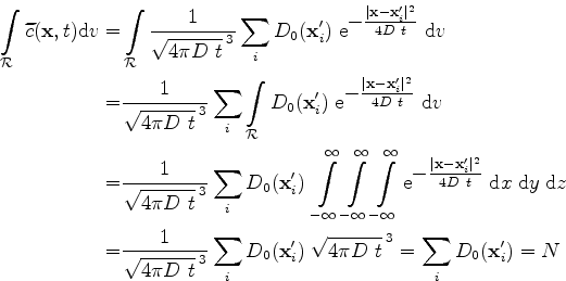$$\begin{gather*}\begin{split}\int\limits_\mathcal{R} \widetilde{c}({\mathrm{\bf x... ...pi D t}^{\;3} = \sum_i D_0 ({\mathrm{\bf x}}_i') = N \end{split}\end{gather*}$$ (4.8)

is preserved, too. The preservation of the implanted dose is a significant and necessary condition for the quality of the method. In total, the amount of implanted ions must not change during the diffusion process. Therefore, the discrete formulation must fulfill this preservation, too.

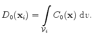
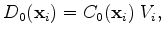
Since the implantation distribution is delivered on a grid, this grid can be used for calculating the entire dopant diffusion process. In this case, the initial dopant concentration $D_0({\mathrm{\bf x}}_i)$ is defined on the grid points $p_i$ and therefore, the integration of (4.5) can be omitted and replaced by

$$D_0({\mathrm{\bf x}}_i)=C_0({\mathrm{\bf x}}_i) \; V_i,$$ (4.9)

which is the initial concentration at the grid point, weighted by the control volume of the Voronoi box.