1.2 Influence of the Simulation Grid
on the Solution

In the following the influence of two different grid refining methods will be compared. The first method refines the grid by a global unstructured increase of grid points. This is done by down-scaling the maximum grid element area. This approach will be compared to a more sophisticated point placement algorithm which, as will be shown, also achieves more accurate results.

Figure 1.1: The simulation domain of the coaxial capacitor.

In Figure 1.1 a quarter of the cross-section of a coaxial capacitor is shown. The electrode areas $\partial B_{1}$ and $\partial B_{3}$ are biased at 0  V and 1  V, respectively. The whole capacitor area $B$ is filled by an insulator with constant permittivity $\varepsilon$.

Because of the axial symmetry of the device, this simulation could be performed in one dimension. However, to compare the influence of the grid adaption methods, the simulation is performed in two dimensions. This artificial example is chosen, because the analytical solution of this problem can be easily found and can be used to calculate the error of the two grid adaption methods.

For the analytical and numerical evaluation of this problem, the Laplace equation [22]

$$- \operatorname{div}( \varepsilon \;\operatorname{grad}\phi) = 0$$ (1.1)

has to be solved within the domain $B$. The boundary conditions are

$$\phi=0 \mathrm{V} \partial B_{1}$$ (1.2)

$$\phi=1 \mathrm{V} \partial B_{3}$$ (1.3)

Since only a quarter of the whole coaxial capacitor is simulated, vanishing normal derivatives at the radial boundaries have to be appended

$$\partial_n \phi= 0 \partial B_{2} \partial B_{4}$$ (1.4)

For this simple structure, an analytical solution can be found and the electrostatic potential results to

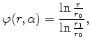$$\phi(r,\alpha) = \frac{\ln \frac{r}{r_0}}{\ln \frac{r_1}{r_0}},$$ (1.5)

only depending on the distance $r$ from the center and independent of the radial angle $\alpha$. The symbol $r_0$ denotes the radius of the inner electrode and $r_1$ of the outer one.

Within the following Box Integration simulations, the error of the discrete approximations is defined as:

$$f = \vert\;\phi- \overline{\phi}\;\vert _\mathrm{max}.$$ (1.6)

The symbol $\phi$ represents the exact analytic solution. In consistency with the Box Integration method, the numerical approximation $\overline{\phi}$ is derived by linear interpolation inside the triangles of the grid.

The first meshing method places the grid points with nearly constant grid density. The only constraint for the grid density is a maximum allowable triangle area, to achieve the different grid densities. A typical grid produced by the Delaunay triangulator triangle [61] is shown in Figure 1.2.

Figure 1.2: Unstructured grid refinement, 237 grid points. The resulting maximal discretization error is 134  mV.

Figure 1.3: Refinement, which is adapted to the given problem, $17 \times 14$ grid points. The maximal discretization error is reduced to 8.7  mV.

The adapted grid generation method places the grid points quasi-orthogonally (Figure 1.3), which means a constant number of points $m$ with equidistant point spacings along the expected equipotential surfaces (lines with constant radius) and a constant number of grid points $n$ with radially increasing point distances in the perpendicular direction (along the diametric lines). This way, the number of grid points along and across the radial lines can be varied arbitrarily. The resulting grid is a triangular grid with $m \times n$ grid points. Figure 1.2 and Figure 1.3 contain approximately the same number of grid points.

In Figure 1.4 the error of the numerical solution on the adapted grid with $10$, $20$, $30, \ldots, 60$ ticks in radial direction, as a function of the total number of grid points is displayed. An interesting aspect derived by this error analysis is that the error reaches a minimal value, if the tangential and radial number of grid ticks lie within the same value. In this example for instance exactly at $30 \times 34$ grid ticks, but also verified by trials with other numbers of radial and tangential ticks. An additional increase of tangential sampling points does not improve the solution.

Figure 1.4: Error of the adapted grid. Each curve results from a grid with $n$ ticks in radial direction. The total number of grid points is varied. A minimal error is reached, if the number of radial and tangential ticks are nearly of equal size.

Figure 1.5: Errors of the unstructured versus the adapted grid. The unstructured grid is refined by a maximum area constraint. The adapted grid generation is built with the same number of grid ticks in radial and tangential direction.

By varying the number of ticks radially and axially, the error depending on the total number of grid points is compared to the unstructured method. This can bee seen in Figure 1.5. The conclusion is, as expected, that within the adapted point placement the error differs by orders of magnitude. Within the simulation range of grid points an error dependency of $f \propto n^{-0.8}$ can be expected for the unstructured method and about $f \propto n^{-1.1}$ for the more sophisticated method.

Thus, the evaluation of the numerical solution on the unstructured grid needs about $10$ times the number of grid points than the improved version to achieve equal accuracy -- also implicating the same factor for memory and time consumption. Within three-dimensional simulations this aspect becomes even more severe.