|
|
|
|
Previous: 3.3.3 Non-MAXWELLian Distributions Up: 3.3 Supply Function Modeling Next: 3.4 The Energy Barrier |
|
|
|
|
Previous: 3.3.3 Non-MAXWELLian Distributions Up: 3.3 Supply Function Modeling Next: 3.4 The Energy Barrier |
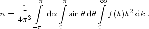
| (3.37) |
 |
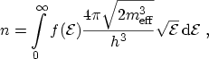
(3.38) |
 |
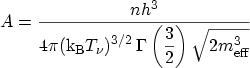
(3.39) |
 |
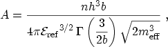
(3.40) |
 |
(3.41) |
 |
(3.42) |
|
|
|
|
Previous: 3.3.3 Non-MAXWELLian Distributions Up: 3.3 Supply Function Modeling Next: 3.4 The Energy Barrier |